Fun with Frequencies and Gradients!

Part 1: Frequency Domain

Part 1.1: Warmup

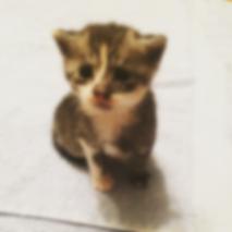
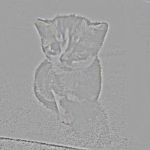
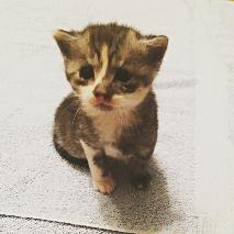
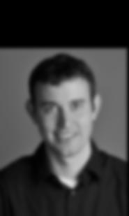
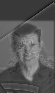
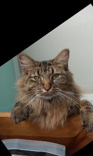
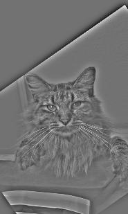
For this portion, we implemented the unsharp masking technique. The process of doing so is:

1. Use a Gaussian ("low pass") filter on the image that you want to sharpen. This result will be a blurry version of your image.
2. Subtract the blurry image from the original to get the high frequency details of your image.
3. Multiply the high frequency image by some small scalar (less than 1) and add it to your original. The result is your sharpened image!

Here we have included images from sharpening an image of a kitty: (The effects are subtle, but is perhaps the most noticeable in the carpet detailing)

Original image	Gaussian filtered image (i.e. low pass filtered image)	Subtracting Gaussian filtered image from original (i.e. high pass filtered image)	Resulting sharpened image

Part 1.2: Hybrid Images

In this portion, we created hybrid images by taking the high frequencies from one image and adding the low frequencies from another image. At closer distances, the high frequencies are more noticeable. At further distances, the low frequencies are more noticeable.

The way we get the low frequencies is by using a low pass filter like the Gaussian filter from part 1.1. Similarly, we get the high frequencies by using a high pass filter like the Laplacian filter from 1.1. (The Laplacian filter is simply the impulse/identity filter minus the Gaussian filter, and is done in part 2 of 1.1)

Here is a pair of sample images that we worked with to demonstrate this concept:

Original image of Derek	Low pass filtered Derek
Original image of Nutmeg	High pass filtered Nutmeg	Hybrid image of Derek and Nutmeg

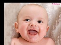
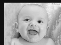
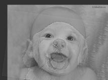
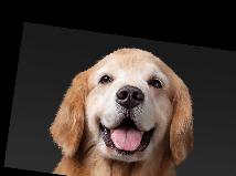
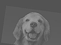
Here is a blend of a golden retriever and a baby: (Notice that the hybrid is quite unconvincing. This is largely because we are doing global alignment instead of localized alignment. In this case, the eyes and nose is aligned, but the mouth and the rest of the head is not aligned.)

Original image of baby	Low pass filtered baby
Original image of golden retriever	High pass filtered golden retriever	Hybrid image of baby and golden retriever

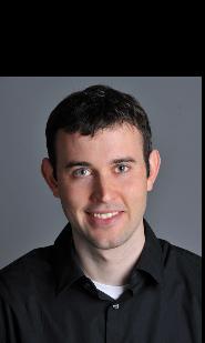
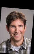
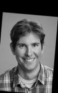
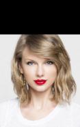
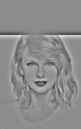
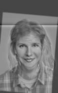
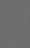
Included here is a blend of one of UC Berkeley's professors and Taylor Swift: (This hybrid is surprisingly convincing!)

Original image of Prof. Denero	Low pass filtered Prof. Denero
Original image of Taylor Swift	High pass filtered Taylor Swift	Hybrid image of Prof. Denero and Taylor Swift

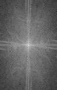
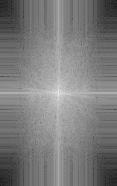
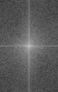
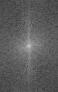
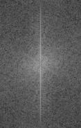
For the blend of Professor Denero and Taylor Swift, we also included the log magnitude of the Fourier transform of each of the images displayed above:

FFT of original image of Prof. Denero	FFT of low pass filtered Prof. Denero
FFT of original image of Taylor Swift	FFT of high pass filtered Taylor Swift	FFT of hybrid image of Prof. Denero and Taylor Swift

Part 1.3: Gaussian and Laplacian Stacks

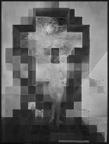
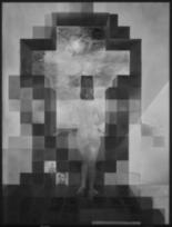
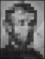
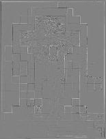
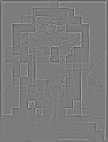
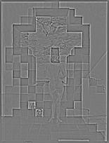
This part is dedicated to creating Gaussian and Laplacian stacks. A Gaussian stack is created by repeatedly applying a low pass filter to an image. The Laplacian stack can be created by subtracting neighboring layers of a Gaussian stack. The final layer in the Laplacian stack contains the low pass image used in the last subtraction.

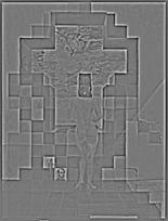
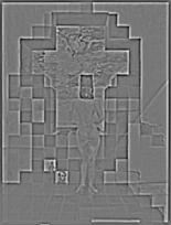
A Gaussian stack and Laplacian stack was created for Salvador Dali's painting of Lincoln: (Notice that the last image in the stack is the residual low pass filtered image used in constructing the Laplacian stack.)

Gaussian stack for Lincoln

Laplacian stack for Lincoln

This was also done from the Professor Denero and Taylor Swift blend that we had in the previous section:

Gaussian stack for Denero + Swift

Laplacian stack for Denero + Swift

Part 1.4: Multiresolution Blending

The process of multi-resolution blending is as follows...

1. split your two images into bands of image frequencies (i.e. get the Laplacian stack of both images),
2. blend the images at each band with your low pass filtered mask where the degree of blurriness of your mask varies depending on the band of image frequency,
3. and add the blended bands together to get your final image.

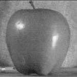
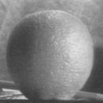
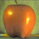
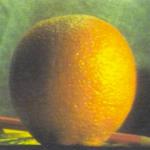
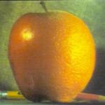
Here, we demonstrate multiresolution blending with a vertical seam/mask:

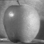Apple (left side of blended image)	Orange (right side of blended image)	Oraple (blended image)

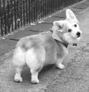
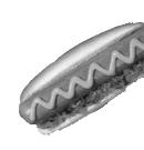
Here, we demonstrate multiresolution blending with an irregular mask: (Notice that since the images are not well aligned, this blending is extremely unconvincing.)

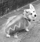Corgi (base of blended image)	Hotdog	Hotdog-corgi (blended image)

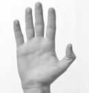
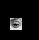
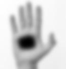
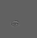
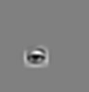
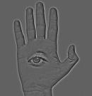
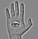
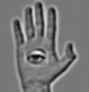
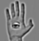
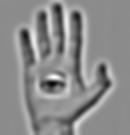
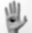
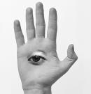
Here is another multiresolution blending with an irregular mask: (Also included are the individual layers that went into creating this image. Disclaimer: they are a bit eery to look at for long periods of time.)

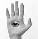Hand (outside of blended image)	Eye (inside of blended image)	Hand-eye (blended image)

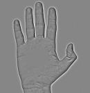
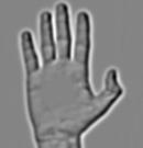
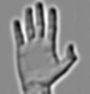
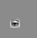
Laplacian stack for the masked bands of the hand image
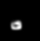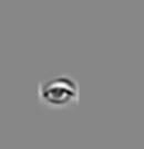
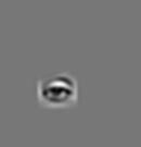
Laplacian stack for the masked bands of the eye image
Laplacian stack for sum of the two corresponding bands of the masked hand image and the masked eye image

Bells and Whistles (Colored Multiresolution Blending)

We've only seen multiresolution blending in black and white so far, but we can also do it in color! The idea is to apply our multiresolution blending technique from above to each of the color channels. Then we can add the blended color channels together.

Colored apple (left side of blended image)	Colored orange (right side of blended image)	Colored oraple (blended image)

Part 2: Gradient Domain Fusion

The main idea of gradient domain fusion is that we will exploit the fact that people care much more about the gradient of an image than the overall intensity. Suppose we want to blend some target into a source image. The pixels in the source image that do not overlap with the target, we can keep the same. We can solve for the values of the overlapping pixels by formulating it as a least squares problem.

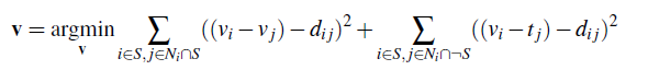
Denote the source region as "S" and the target region as "t". We want to solve for the intensity values "v". Then we choose "v" to be

where "i" is a pixel in the source region and "j" is a 4-neighbor of "i". Intuitively, we can think of this as we have gradients from the target image that we want to include in the source image, and we will find the set of pixels that best incorporates both the gradients from the target image and that of the source image so there isn't a harsh seam between the two regions.

Part 2.1: Toy Problem

For this part, we simply wanted to demonstrate the effectiveness of this technique. We simply tried to reconstruct an image from its gradients. In relation to the equation above, there is no distinction between the target and the source image. Additionally, we will not be looking at the 4-neighbors of the pixels we are solving for, but instead we will look at 2 of its neighbors - one in the x-direction and another in the y-direction.

We sought to reconstruct an image of Buzz Lightyear and Woody from Toy Story. Here are our results:

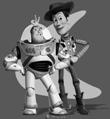Original image	Reconstructed image using gradient domain fusion

Part 2.2: Poisson Blending

Using the technique described in part 2 (i.e. solving for "v" with least squares), we blended several images.

Here are blended sample images of a penguin and climbers:

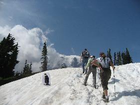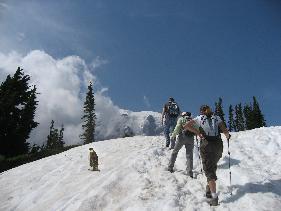Original penguin image	Original climber image	Result of directly copying target image into source	Result of using Poisson blending

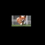
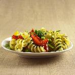
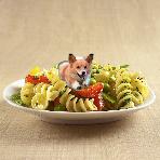
Here, we tried integrating a corgi into a plate of pasta salad:

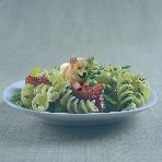Original corgi image	Original plate image	Result of directly copying target image into source	Result of using Poisson blending

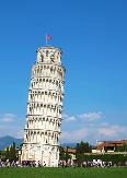
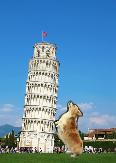
Here, we tried to make a corgi look like it was holding up the leaning tower of Pisa: (Since we are trying to find the best match between the gradients of our corgi and the gradients of our background image, we end up with a sort of weighted average of the two. Unfortunately, this makes our image unconvincing because the corgi is blending into the background.)

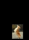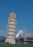Original corgi image	Original plate image	Result of directly copying target image into source	Result of using Poisson blending

Recall the hand and eye image from the multiresolution blending section (Laplacian stack blending). We also blended these images using the Poisson blending technique for comparison. The results are as follows:

Hand (outside of blended image)	Eye (inside of blended image)	Hand-eye using Laplacian stack blending (multiresolution blending)	Hand-eye using Poisson blending

Bells and whistles (Mixed Gradients)

This is a modification to our Poisson blending from above. Our minimization problem becomes

where "d_ij" is the larger of two gradients (target or source gradient) in magnitude. To put it more clearly, if abs(s_i-s_j) > abs(t_i-t_j), then d_ij = s_i-s_j; else d_ij = t_i-t_j.

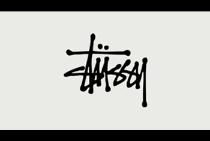
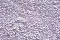
Here, we blended an image of text ("Stussy") onto a textured wall:

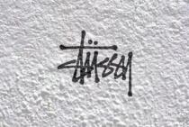Stussy text	Textured wall	Blended result using mixed gradients

Citations

Styling of this page is modified from bettermotherfuckingwebsite.com.