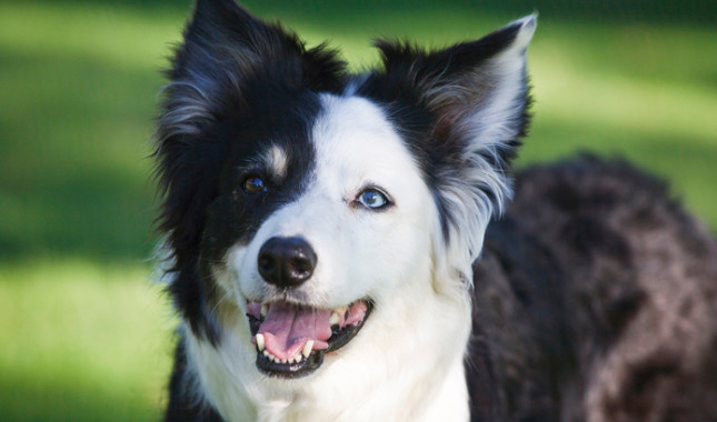
original image of dog
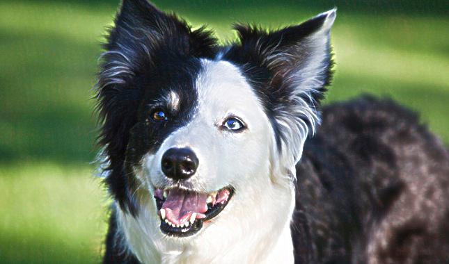
sharpened image of dog
For the image sharpening, I calculated the Laplacian of the image by subtracting the Gaussian (with a sigma value of 3) from the original image, leaving only the edges, which I then added back to the original image to sharpen the edges
original image of dog
sharpened image of dog

original image of Vermeer's Girl with the Pearl Earring
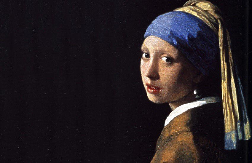
sharpened image of Vermeer's Girl with the Pearl Earring
To create hybrid images, I took the high frequencies of one image using the Laplacian and the low frequencies of another image using the Gaussian filter and combined the images and aligned them such that at far distances, the low frequency image dominates and at close ranges, the high frequency images dominate
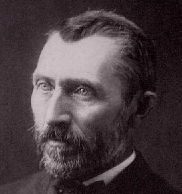
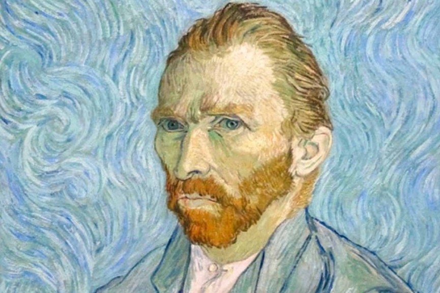
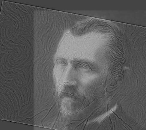
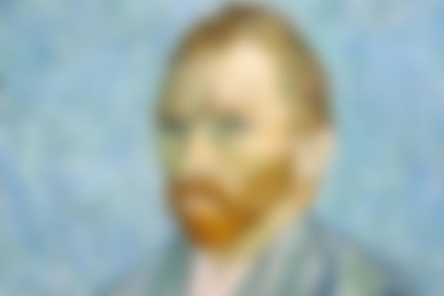
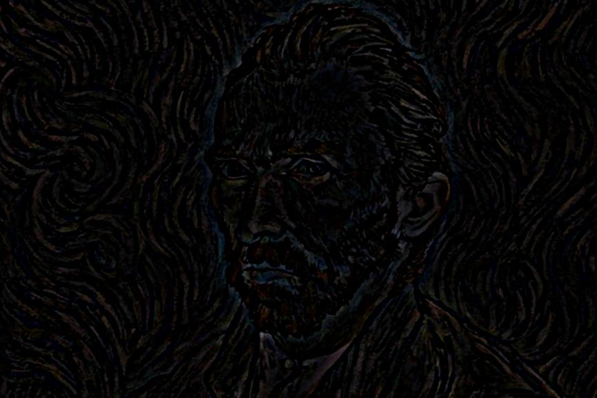
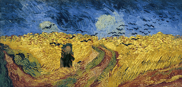
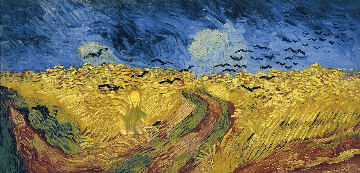
Hybrid of Van Gogh's self portrait and an image of him
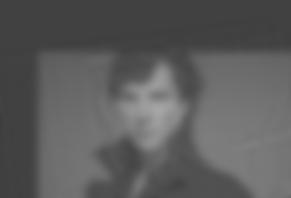
Low frequencies show the photograph of Van Gogh
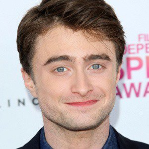
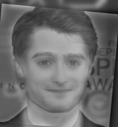
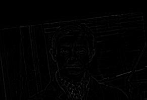
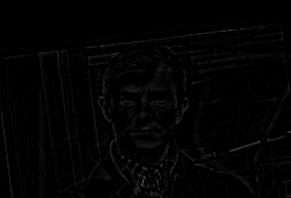
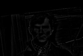
High frequencies look like Daniel Radcliffe
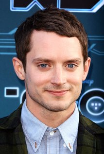
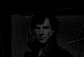
Low frequencies look like Elijah Wood
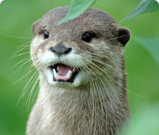
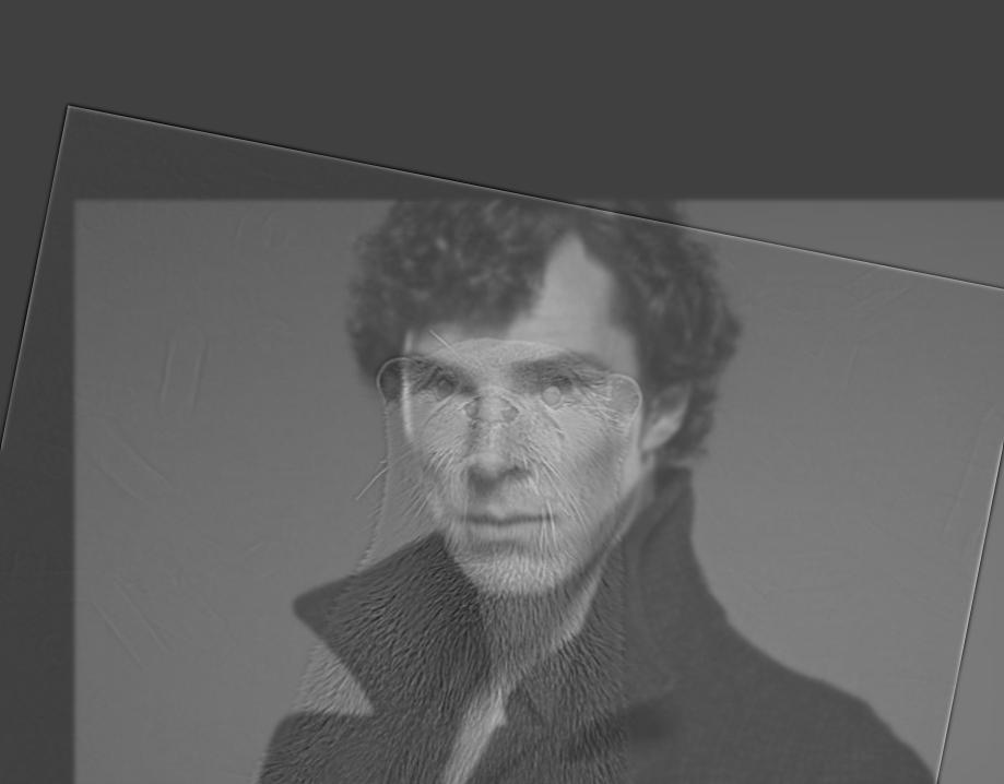
This image failed because the images really couldn't align very well since the face of the otter is much smaller and more squished than Benedict's
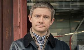

High frequencies show Martin
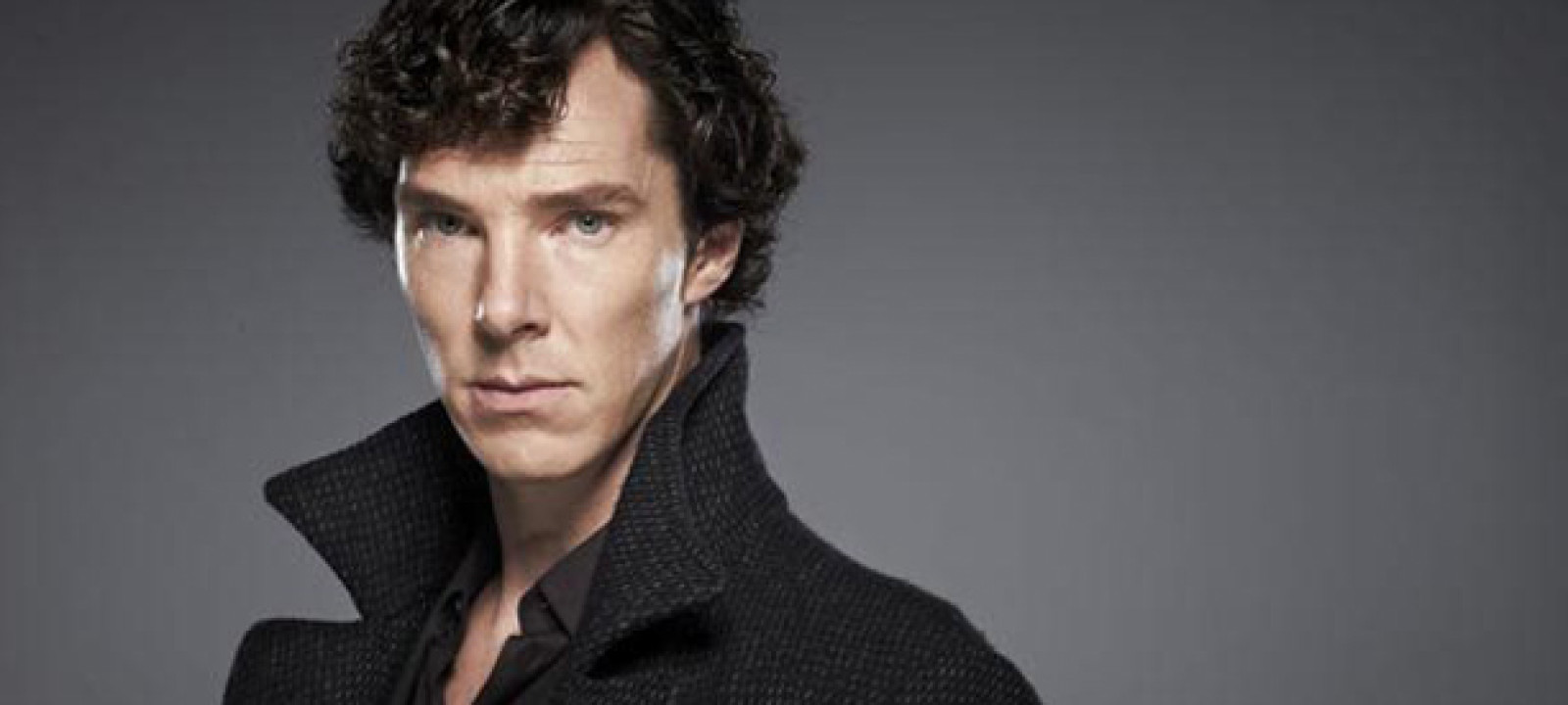
Low Frequencies show Benedict
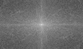
Benedict Frequency
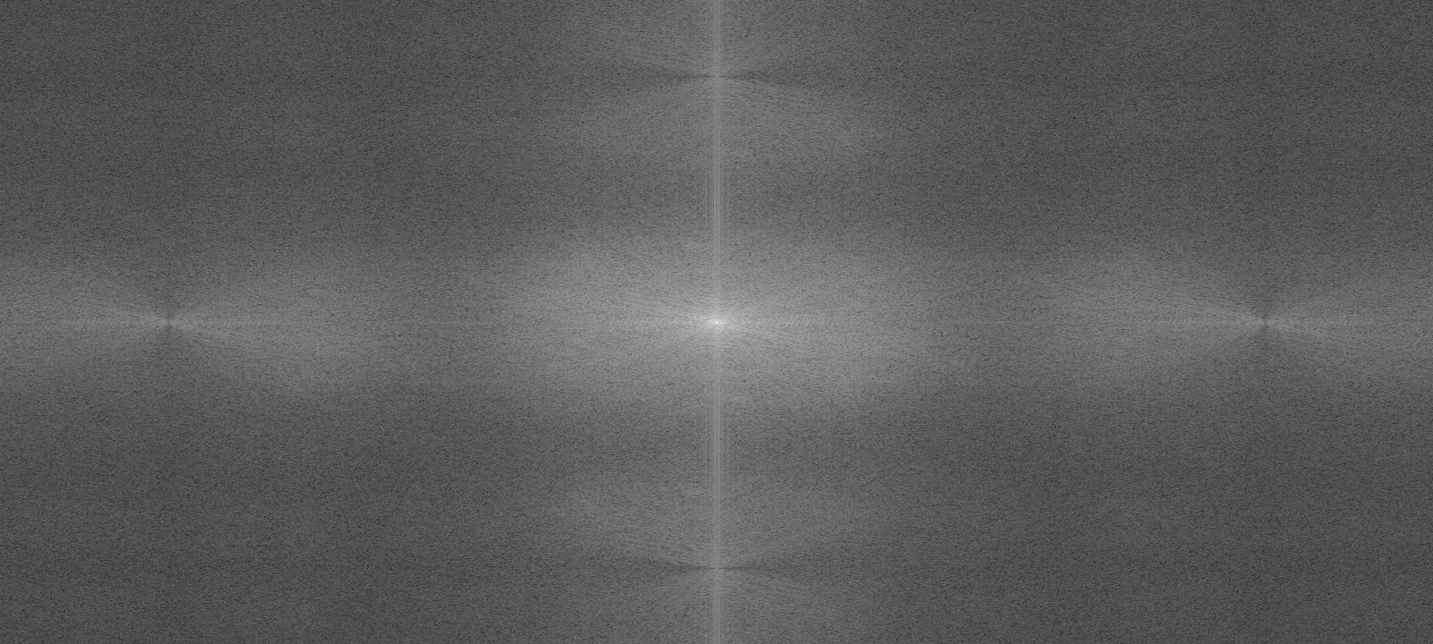
Martin Frequency
Lowpass Frequency
Highpass Frequency
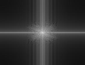
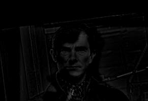
Hybrid Frequency
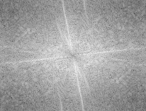
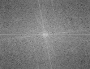
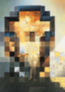
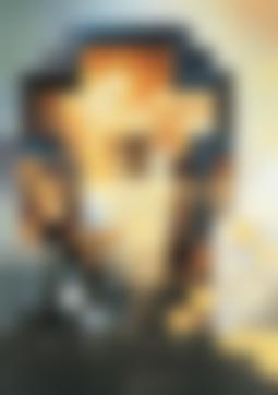
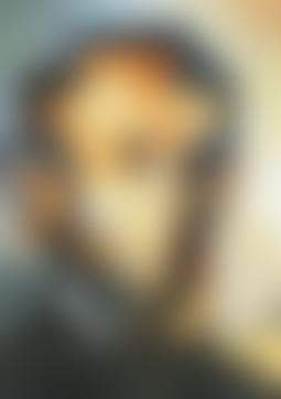
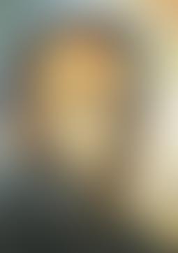
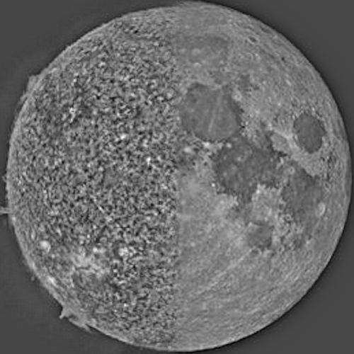
For the Gaussian and Laplacian stacks, I calculated the Gaussians at different sigma values (values of 2, 4, 8, 16, 32) and the Laplacians at those same sigma values, revealing very interesting information about each of the pictures when viewing only the low or high frequency images. For example, in the Dali picture, you can clearly see either Abraham Lincoln or the image with the cross when filtering out frequencies

Original Image of Lincoln by Dali

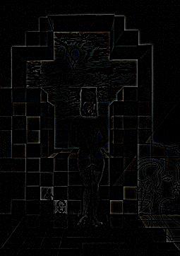
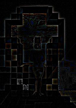
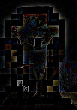
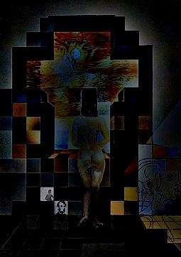
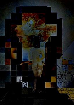
Top row: Gaussian stacks, Bottom row: Laplacian stacks
Original Van Gogh Self-Portrait

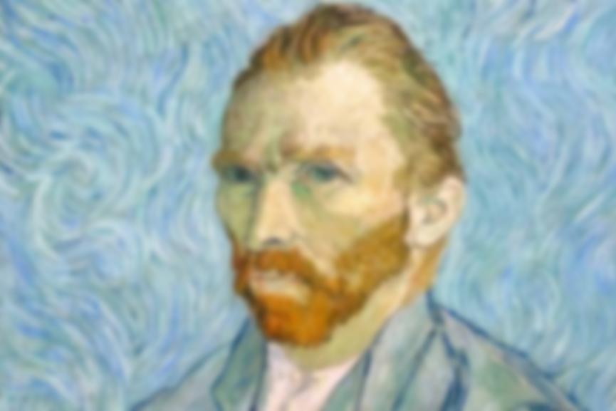


Top row: Gaussian stacks, Bottom row: Laplacian stacks
Original Benedict/Martin


Top row: Gaussian stacks, Bottom row: Laplacian stacks
Multiresolution Blending involved blending together two images by using a mask, blending the images at different levels of Laplacians, and summing the results up. The process was first to obtain two images to blend. Then create a mask that includes the line to blend the images. I then created Laplacian stacks of the two images and added the stacks to each other weighted by the Gaussians of the masks to obtain a final image that was the blended result of the two
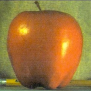
Original Apple
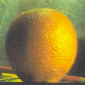
Original Orange

Mask
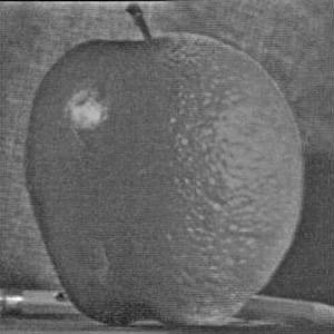
Blended Image
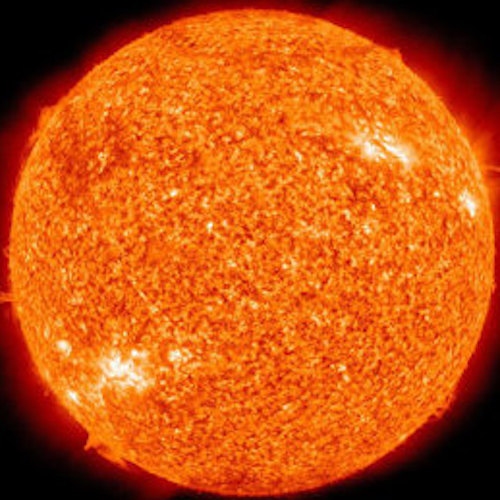
Original Sun
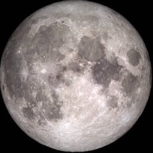
Original Moon

Mask
Blended Image
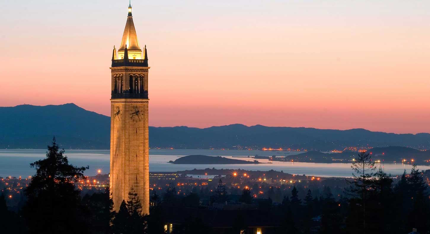
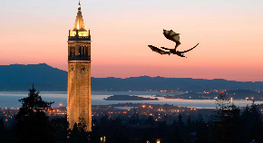
Original Image of Berkeley
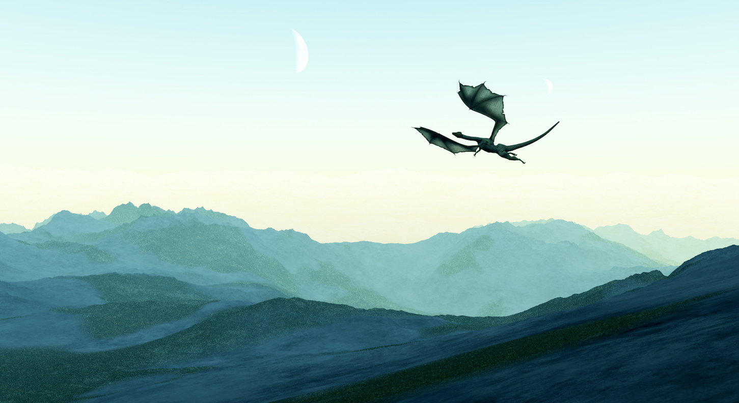
Original Image of Dragon
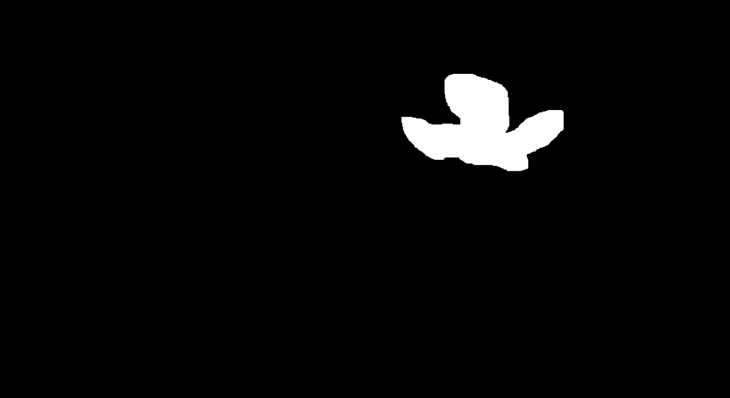
Mask
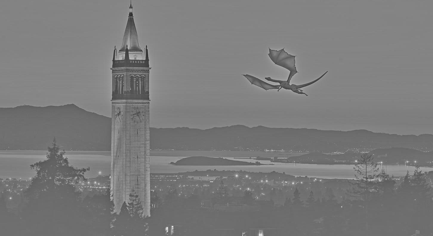
Blended Image
To add color to the images, I blended the three r, g, b channels separately and then combined them together. The images somehow came out rather grayed out though.
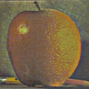
Oraple in Color
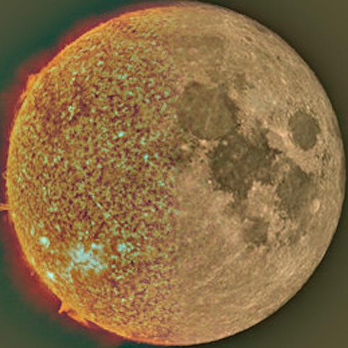
Sun and Moon in Color
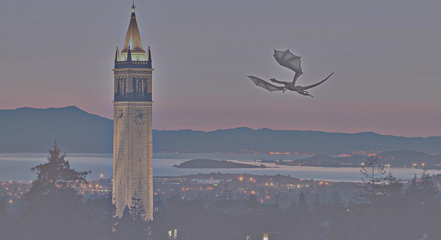
Dragon in Berkeley in Color (ish)
The purpose of the Toy Problem was to practice reconstructing an image by matching the gradients in the source image to the image we are constructing
The objectives were to:
To do this, I used a least squares equation in the form of Ax = b and solving for x to get the values of each pixel of the reconstructed image. Each row in A represented a gradient in either the x or y direction. In the b array, I computed the actual values of the gradients in the source and made sure the reconstructed gradients were equivalent to the source
Original Image
Reconstructed Image
Poisson Blending involved blending images using this equation:

I used a mask to select a region of one image again, and using this equation, came up with the constraints for an A matrix. Essentially, for the area we want to stick our source image S, we want the gradients of the blended image to match the gradients of this source. And for all the areas outside of S, we want the gradients to match those of the target (background) image. That's what the two parts of the equation are maximizing.
In terms of the matrix, for the pixels outside the region S, we want to just take the values from our target image. For the pixels inside S, we want to represent the gradients as an equation of subtraction of the neighboring pixels in our matrix A and in the vector b calculate the value of the source gradient. Then, using scipy.sparse.linalg.spsolve, we can find the pixels of the resulting image.
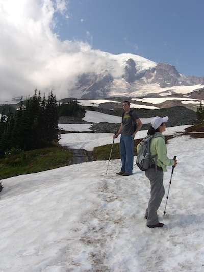
Target Background Image

Penguin to insert

Penguin mask
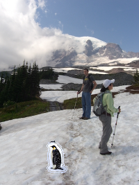
Penguin directly copied
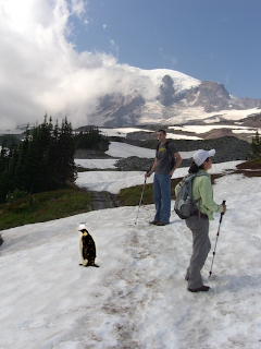
Poisson blending penguin in snow
Target Background Image
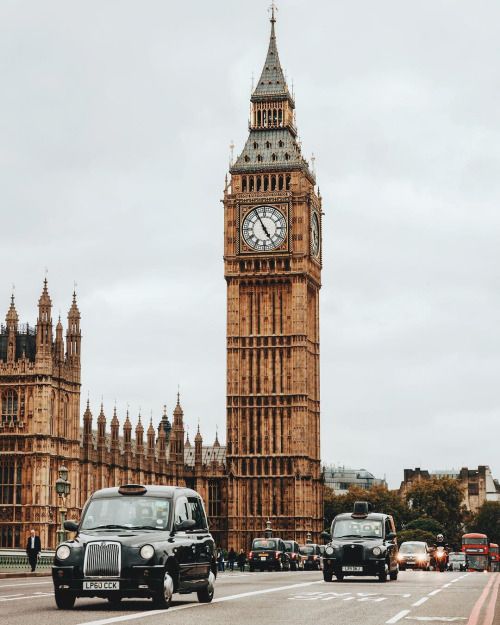
Big Ben to insert
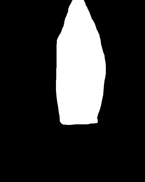
Big Ben mask
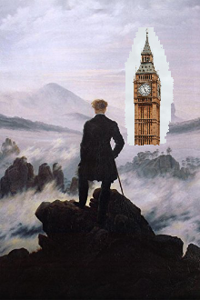
Big Ben directly copied
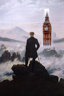
Poisson blending Big Ben
Blending Edvard Munch's Scream into Van Gogh's wheatfield failed because the textures of the paintings, even though they were similar, caused the scream to be almost completely blended into the background

Target Background Image
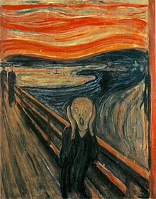
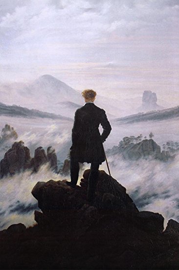
Scream to insert
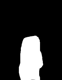
The Scream mask
The scream directly copied
Poisson blending the scream
Taking the image of the dragon over Berkeley, you can see the results of the different types of blending. The colors don't show too well in the multiresolution but, if they had, the blue should still be there in some form, which is gone in gradient-domain fusion. Possion blending is typically better when the blending that needs to be done requires the background to perfectly match the target, as we can also see in the past Van Gogh example where it takes matching the background gradient a bit too far.
Target Background Image
Dragon to insert
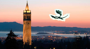
Directly copying
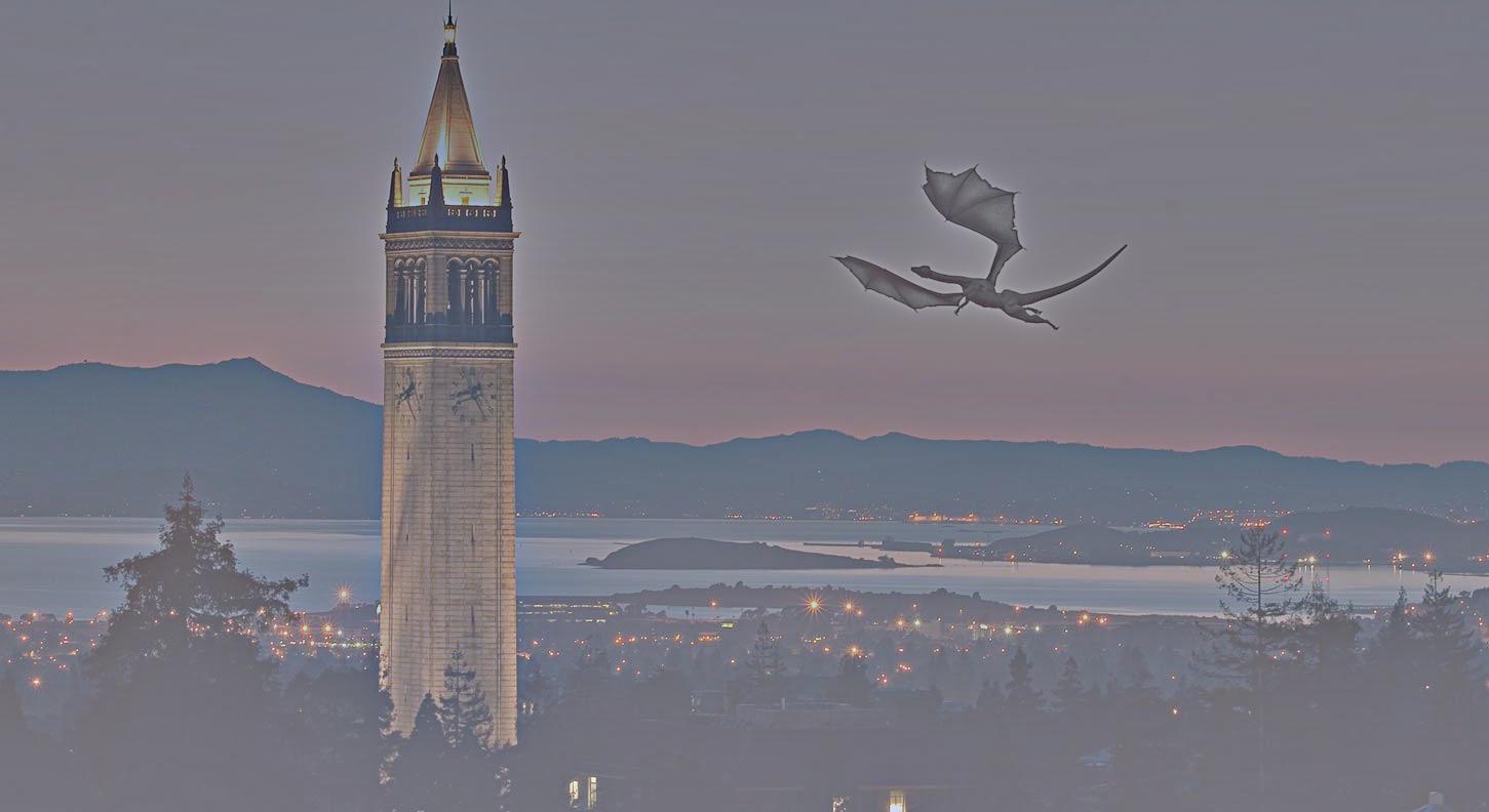
Multiresolution Blending
Poisson blending