
| Original | Sharpened |
|---|---|
|
|
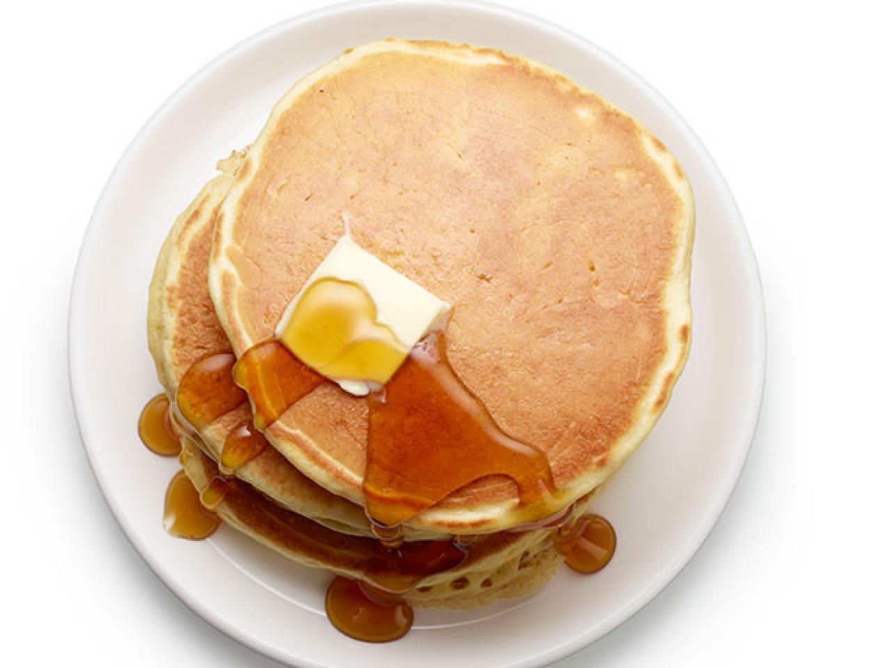
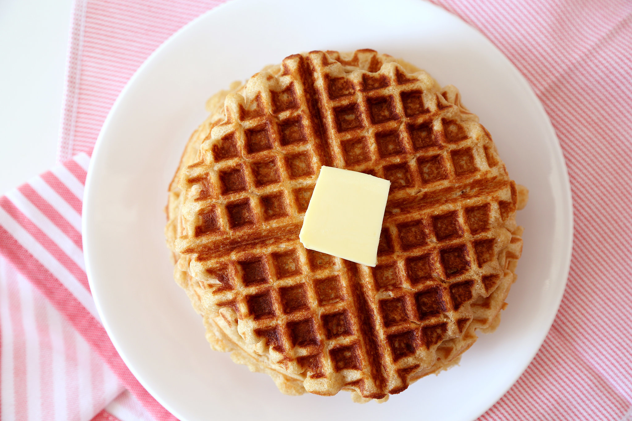
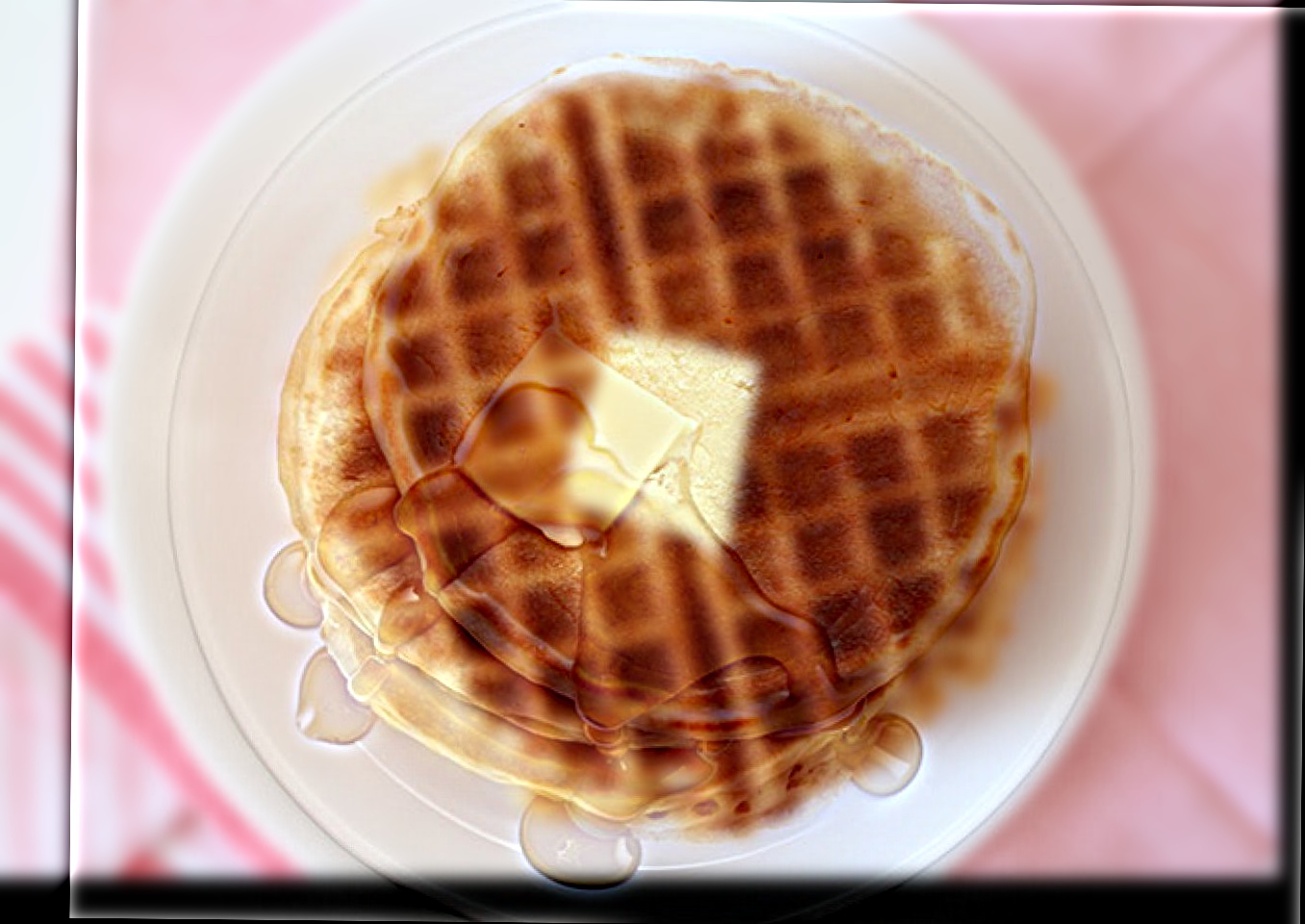
| Image 1 | Image 2 | Hybrid |
|---|---|---|
 |
 |
 |
 |
 |
 |
 |
 |
 |
Above you can see the the pancake + waffle hybrid was a failure case. The pancake image has features mostly in the low frequency range, which get clobbered by the higher frequency features of the waffle image.
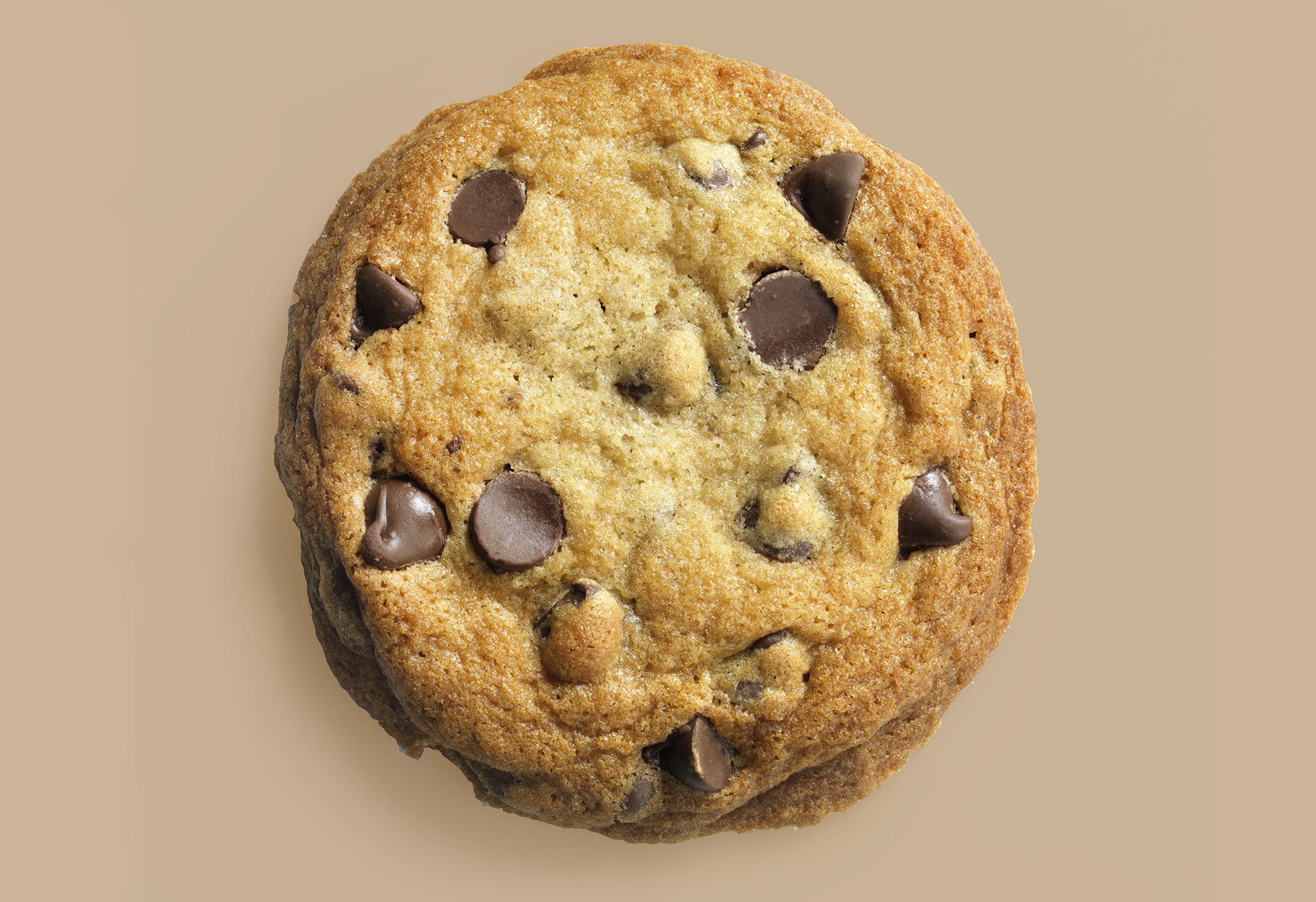
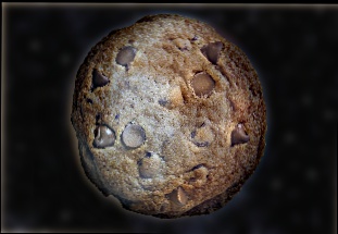
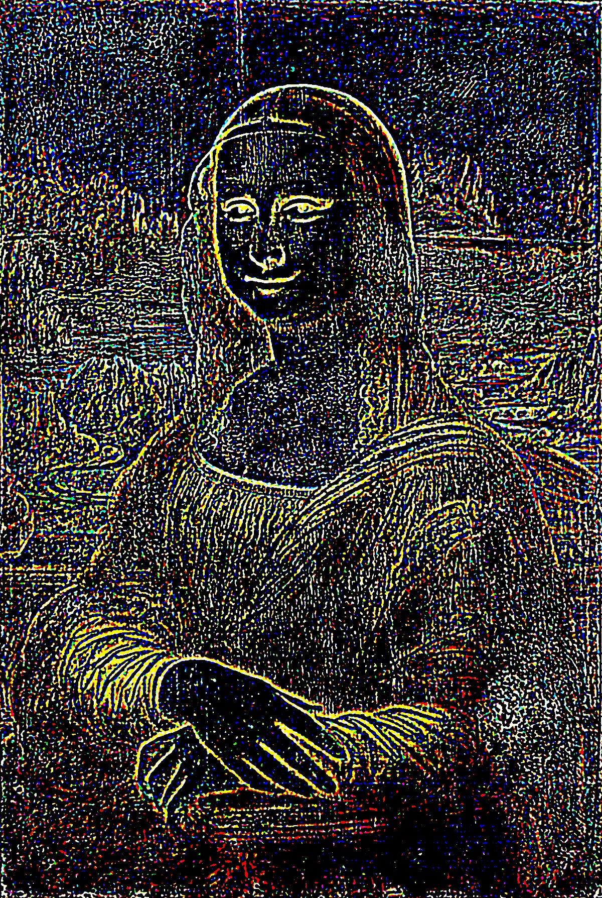
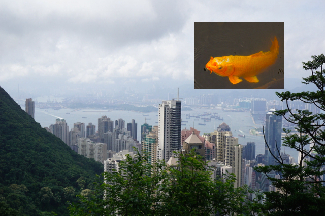
| Image 1 (Cookie) |  |
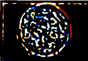
| Image 1 High-Pass |  |
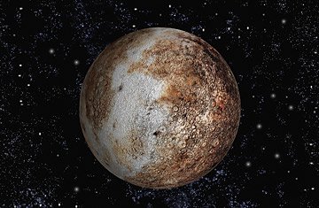
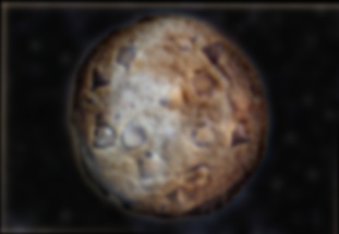
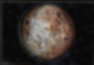
| Image 2 (Pluto) |  |
| Image 2 Low-Pass |  |
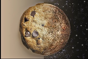
| Image 1 + Image 2 |  |
| Original | 
| ||||
|---|---|---|---|---|---|
| Gaussian Stack |  |
 |
 |
 |
 |
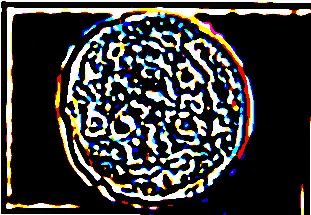
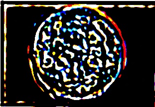
| Laplacian Stack | 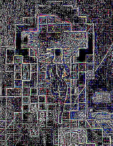 |
 |
 |
 |
 |
| Original | 
| ||||
|---|---|---|---|---|---|
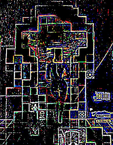
| Gaussian Stack |  |
 |
 |
 |
 |
| Laplacian Stack |  |
 |
 |
 |
 |
| Original |
| ||||
|---|---|---|---|---|---|
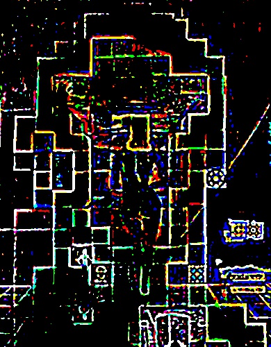
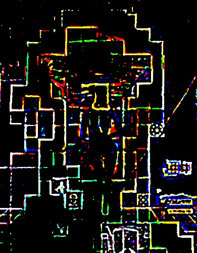
| Gaussian Stack |  |
 |
 |
 |
 |
| Laplacian Stack | 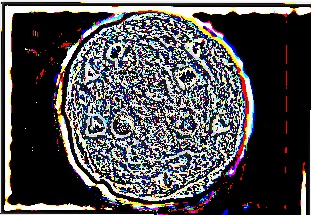 |
 |
 |
 |
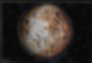 |
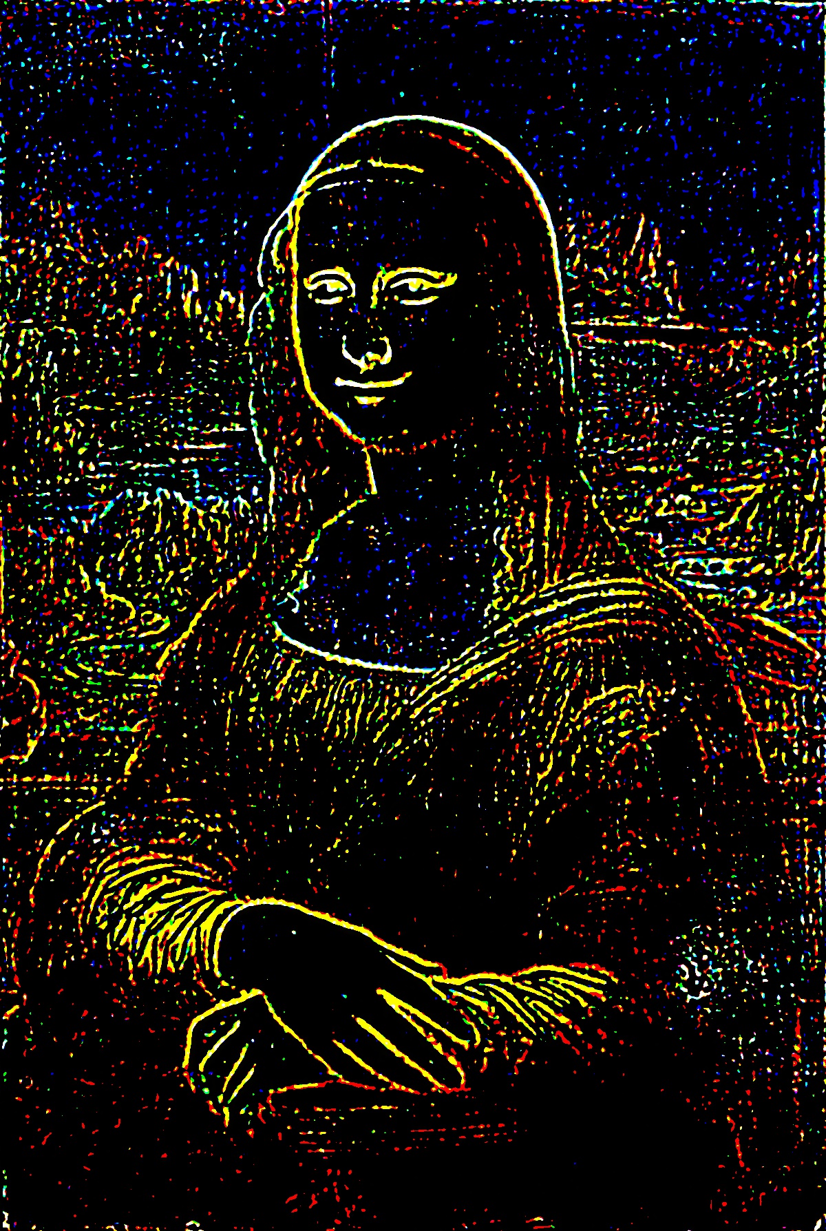
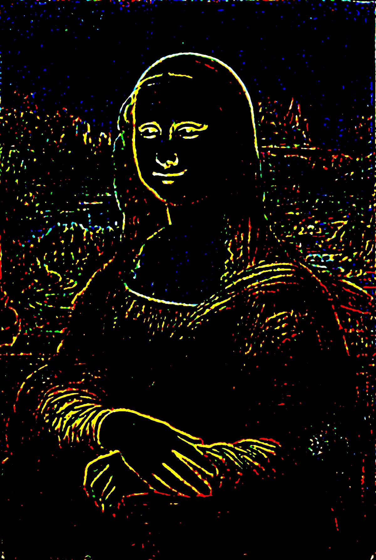
As the Gaussian stack progresses, it becomes more clear that Pluto forms the lower frequencies of the hybrid image. The first few images of the Laplacian stack, on the other hand, show that the cookie composes the higher frequencies of the hybrid image.
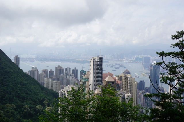
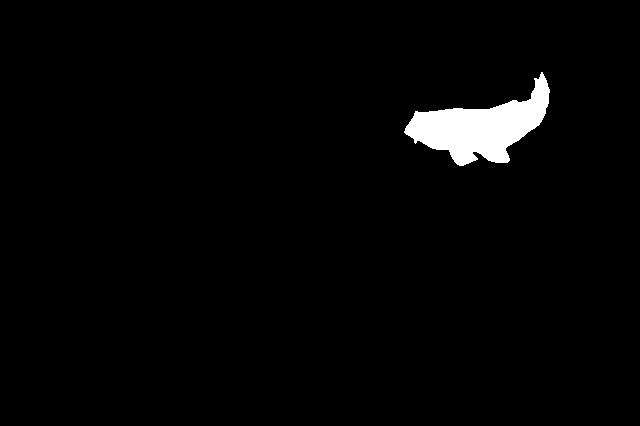
| Image 1 | Image 2 | Mask | Blend |
|---|---|---|---|
 |
 |
 |
 |
|
|
 |
 |
 |
 |
 |
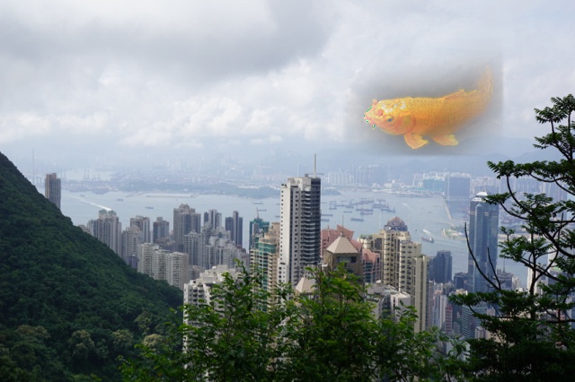 |
Here we implement Poisson blending, a gradient-domain processing technique. Poisson blending aims to seamlessly blend an object or texture from a source image into a target image by finding values of the target pixels the best preserve the gradient of the target image. Such a problem can be modeled as the following least squares problem:

where we want to solve for the new intensity values "v" within the source region "S" (the mask) given the pixel intensities of the source image "s" and the target image "t".
Note that this technique ignores the overall intensity of the source image. This doesn't matter too much because the human eye is not very sensitive to intensity-- the gradients matter more!
| Original | Reconstructed |
|---|---|
 |
 |
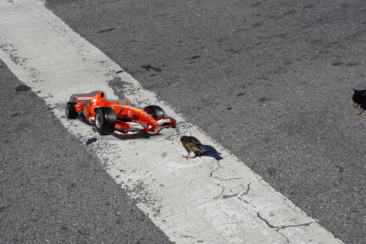
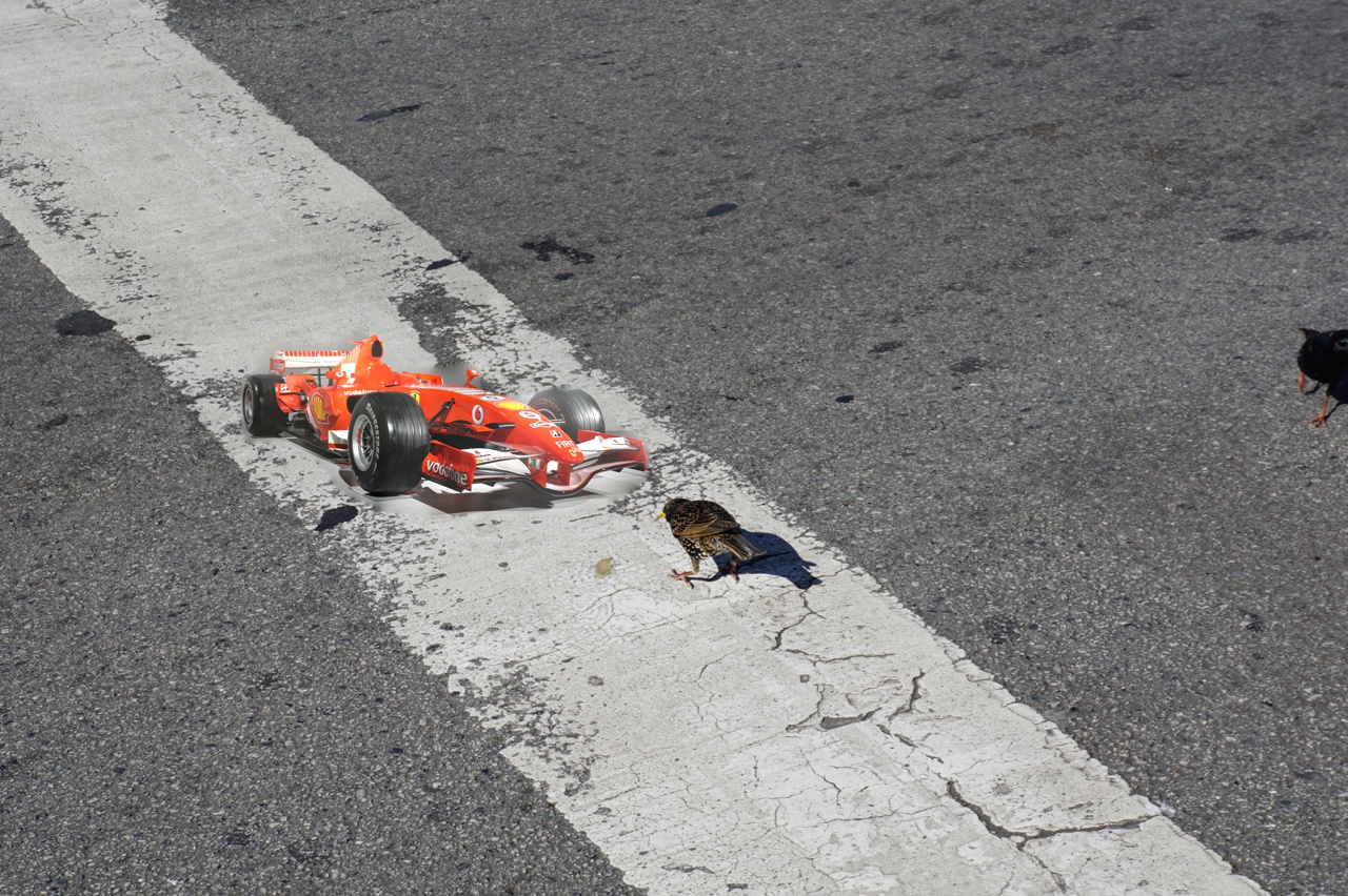
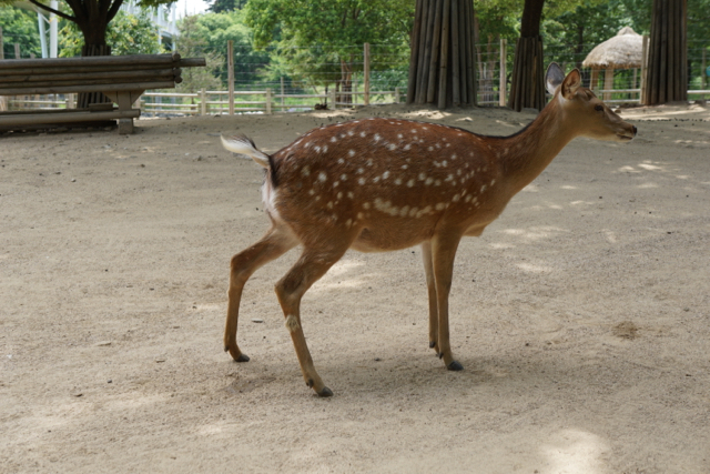
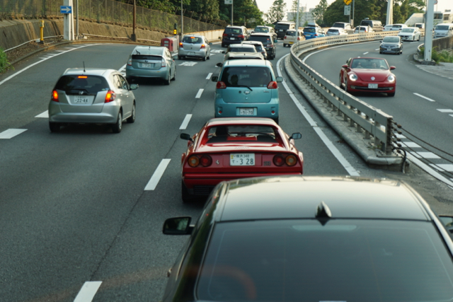
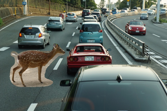
| Source Image | Target Image | Naive Blend | Poisson Blend |
|---|---|---|---|
 |
 |
 |
 |
 |
 |
 |
 |
 |
 |
 |
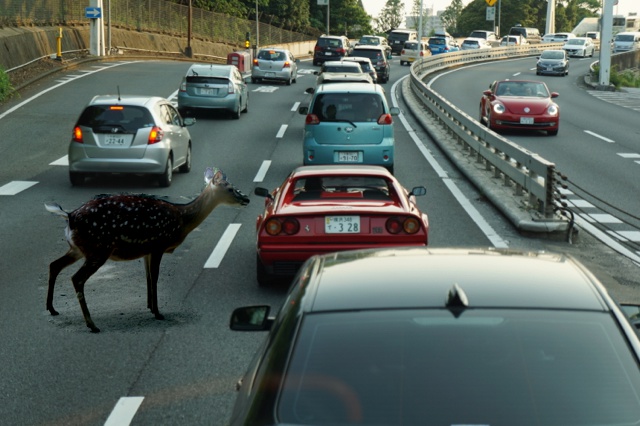 |
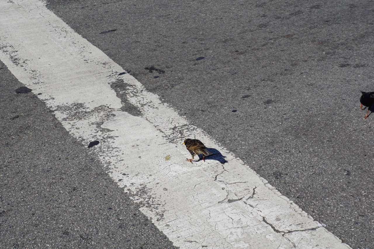
Above, you can see that the deer example was a failure case. The background of the source image (the ground the deer is standing on) differs too much in intensity from the background of the target image (the asphalt road). The Poisson blending technique ignores the original intensity of the source image, so the intensities of the ground are pushed down, and the intensities of the deer pushed down even further. This results in a very dark deer.
One can conclude that Poisson blending techniques only yield good results when the intensities of all three color channels of the source image closely match those of the target image.
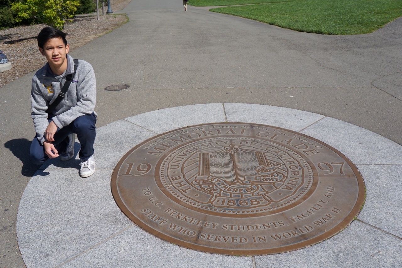
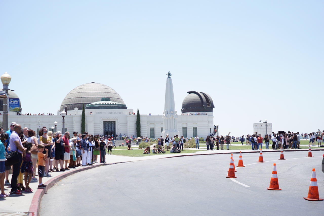
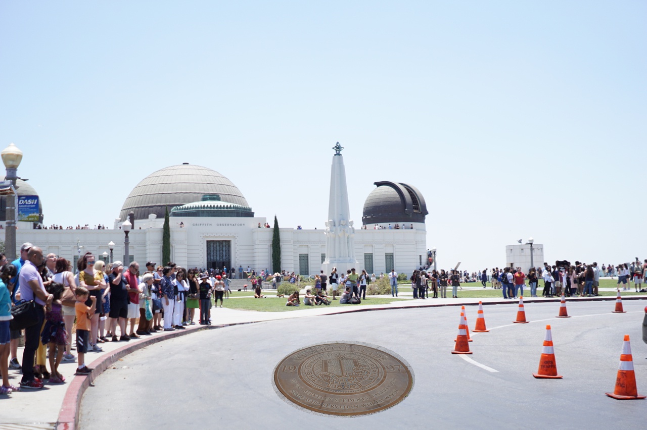
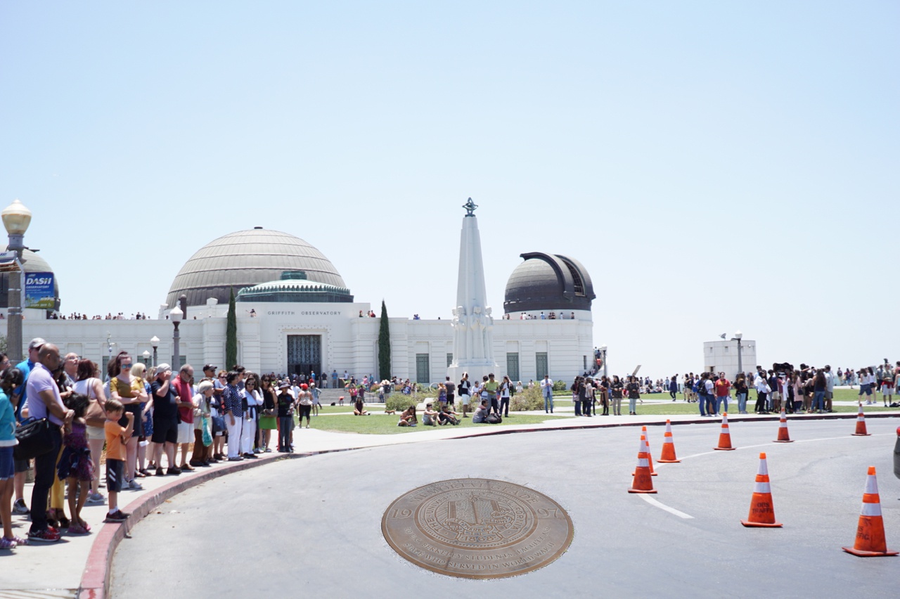
My favorite result is the Berkeley seal superimposed in front of the Griffith Observatory. Although it is not a very interesting example, it shows where Poisson Blending really shines-- when the source and target images closely match.
| Naive | 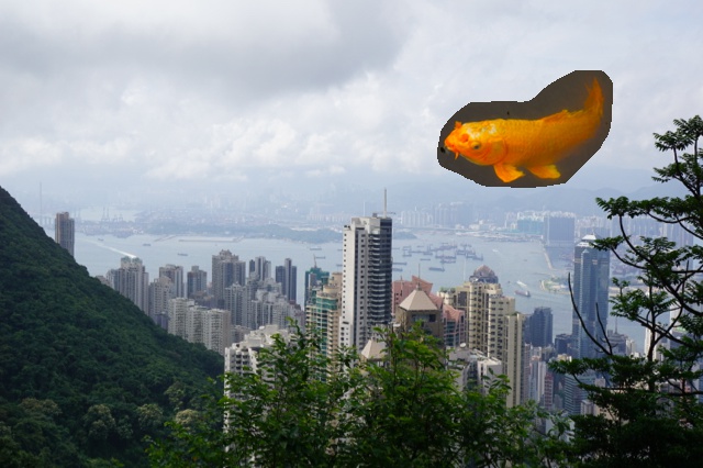 |
| Laplacian Stack Blending | |
| Poisson Blending | 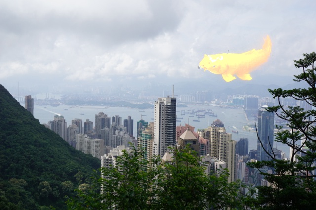 |
| Mixed Gradient Blending |  |
Implementing the Mixed Gradients technique requires a slight modification to the original Poisson Blending problem.
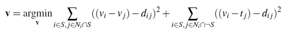
where "d_ij" is the value of the gradient from the source or target image, depending on which has the larger magnitude.
For this type of image, Mixed Gradients offers no improvement over regular Poisson Blending.
Here we implement a better version of skimage's rgb2gray function, which naively converts color to grayscale. To create our so-called "color2gray" function, we first convert the image to HSV (Hue, Saturation, and Value) format. We only use the S and V layers since H only holds the color information. We then approach this as a mixed gradients problem where we want to preserve the maximal gradient between the S and V channels.
| Original | Naive rgb2gray | My color2gray |
|---|---|---|
 |
 |
 |
This project showed me that images are often better or easier to manipulate in other domains such as the frequency domain and the gradient domain. Gradient-domain processing, for example, has a lot of useful applications-- not only for superimposing images on top of other images, but also for creating a better implementation of a color-to-grayscale converter.