Frequencies and Gradients
Jacob Huynh
CS 194-26: Image Manipulation and Computational Photography
Professor Alexei Efros
Overview
As detailed in this paper by MIT professors Oliva, Torralba, and Schyns, hybrid images can be formed by manipulating the high and low frequencies of images. By emphasizing the low frequencies of one image and the high frequencies of another image, we can produce an image that changes with viewing distance. This is all to take advantage of how the human visual system works. Furthermore, in this project we will explore various image blending techniques in order to create realistic renderings of multiple images layered on top of another.
Part 1.1: Image Sharpening
Approach
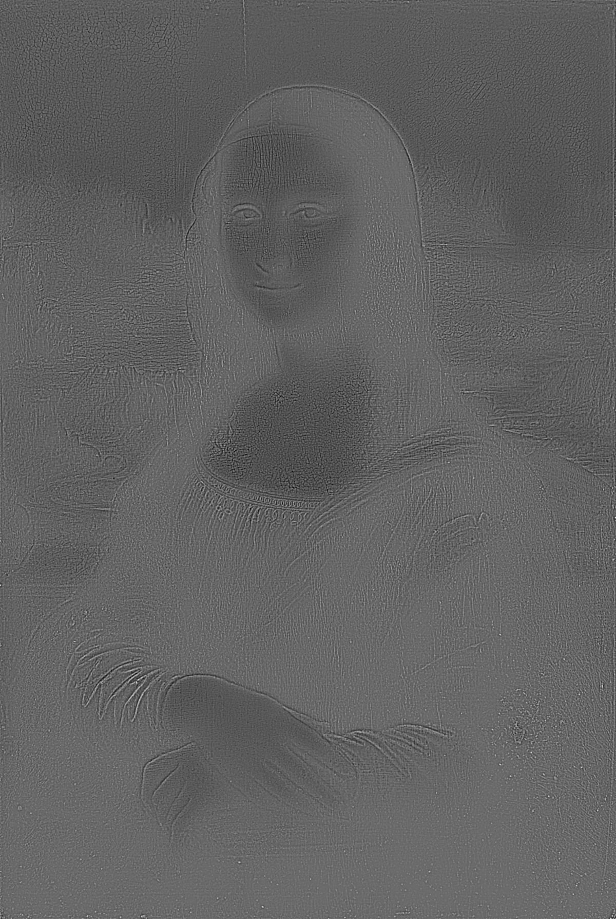
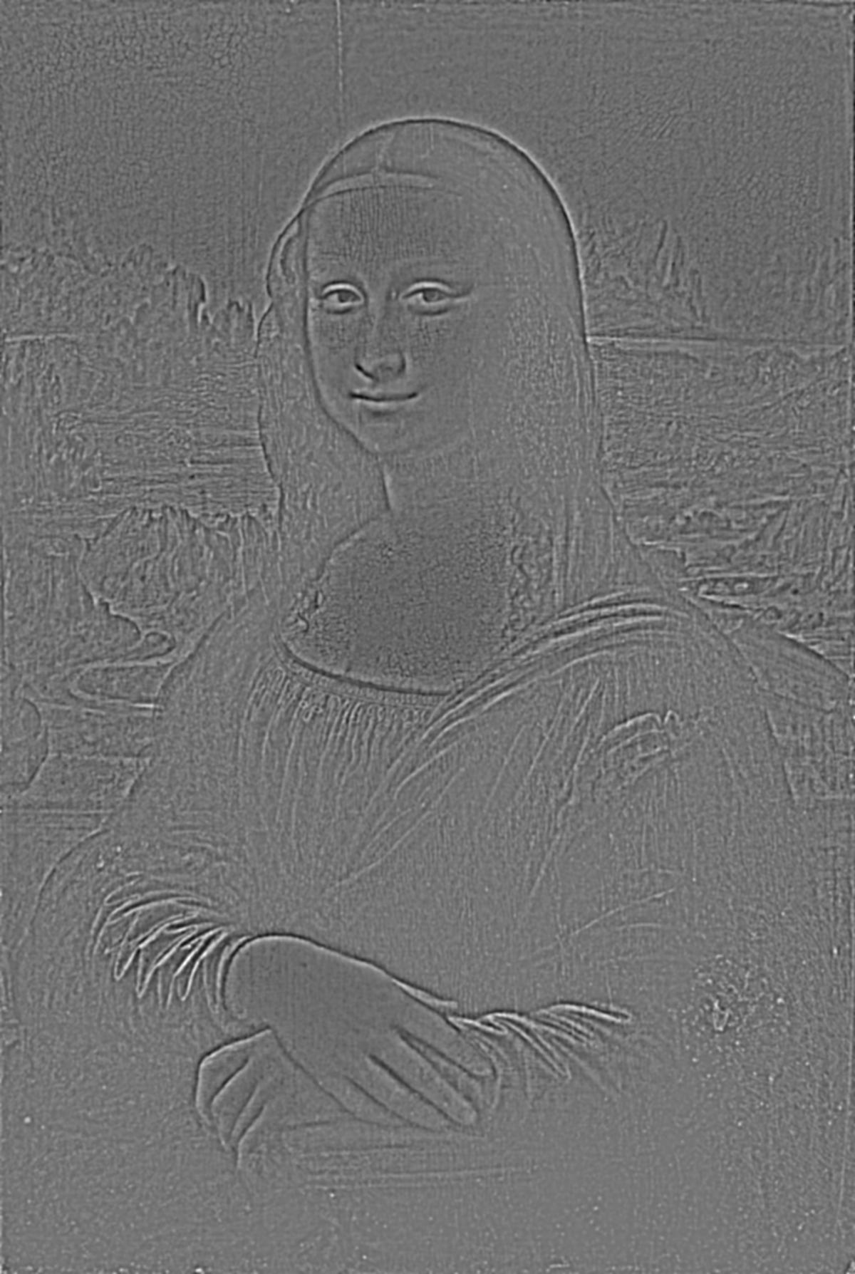
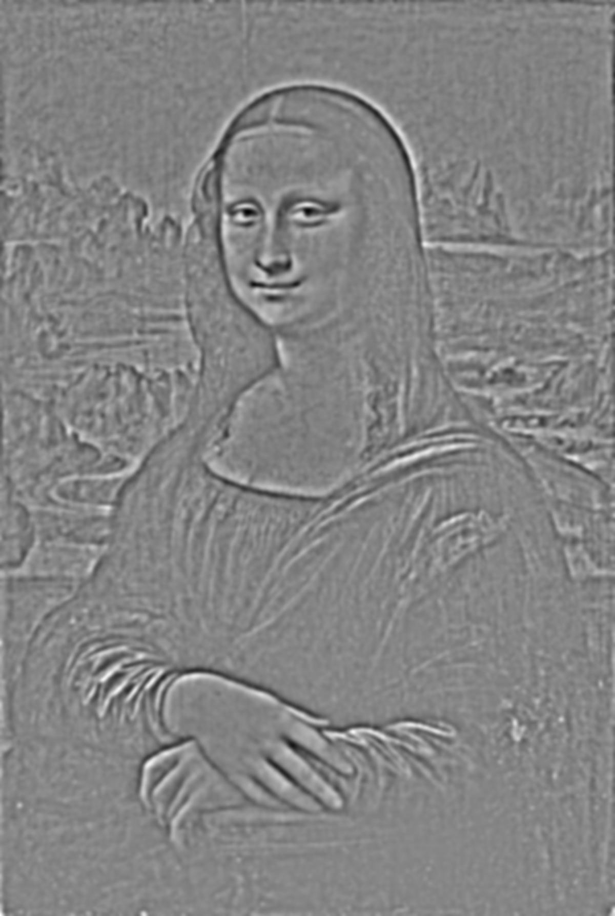
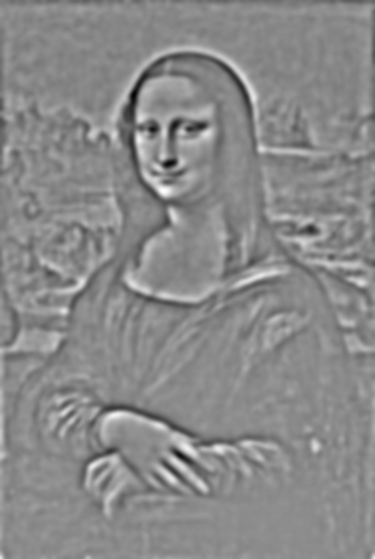
The approach I utilized to achieve this sharpened image was convolving the original image to the unit impulse vector. After that, I simply cropped out the relevant section of the convolution to output the final image. Conversely, I could have also achieved this by blurring the image using a Gaussian filter and then subtracting that blur from the original image. However, I felt that convolving with the unit impulse vector was more straightforward.
original image |

sharpened image |
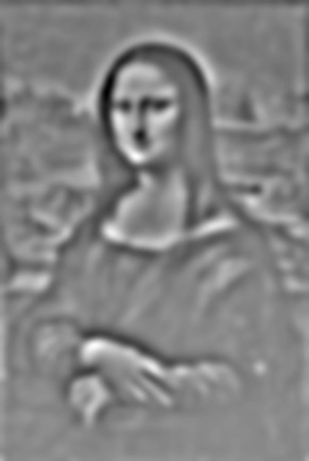
Part 1.2: Hybrid Images
Approach
We can create a hybrid image by following the steps mentioned in the paper above. By using Gaussian filters, we take the high frequency of one image, which will correspond to the picture in the foreground, and add it to the low frequency of another image, which will correspond to the picture in the background. The result is a hybrid image which will display the image with the high pass filter at a close viewing distance and the image with the low pass filter at a further viewing distance.
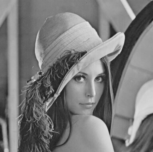
DerekPicture.jpg |
+ |
nutmeg.jpg |
= |
dereknutmeg.jpg |
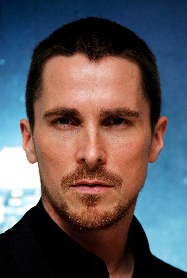
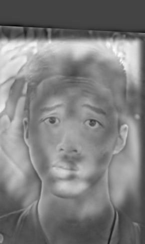
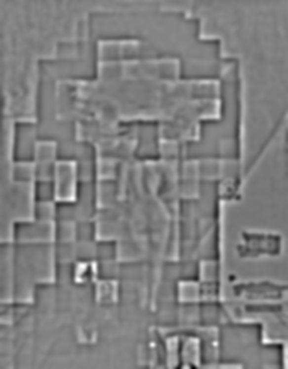
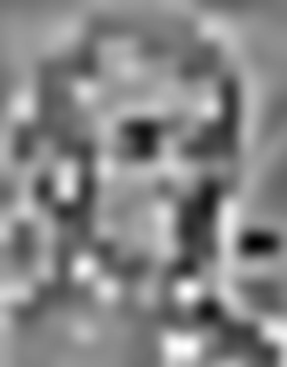
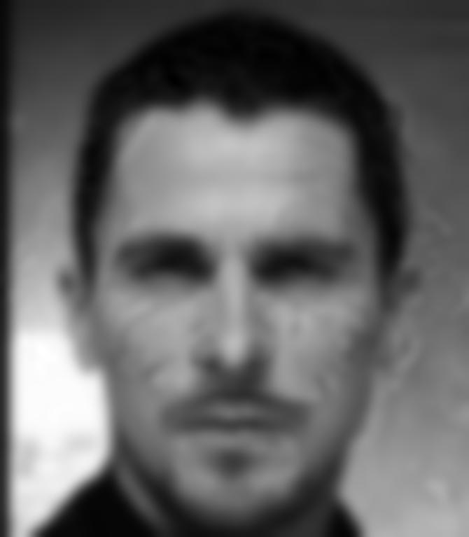
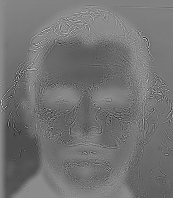
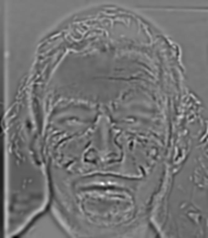
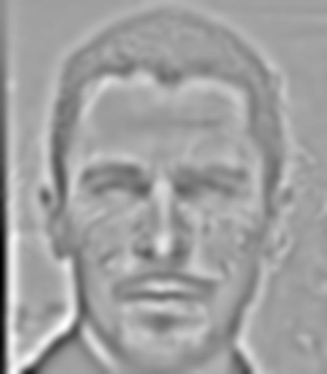
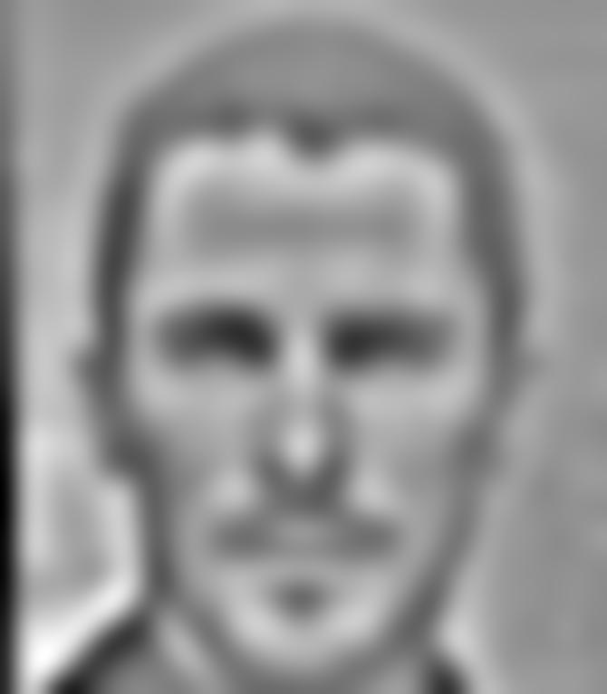
christian_bale.jpg |
+ |

joker.jpg |
= |

christian_joker.jpg |
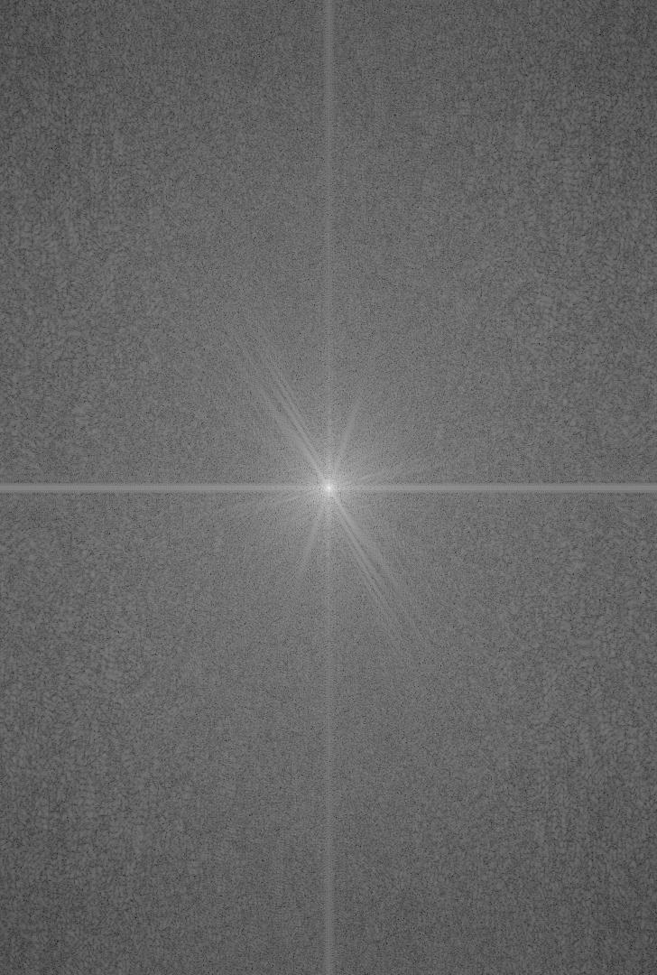
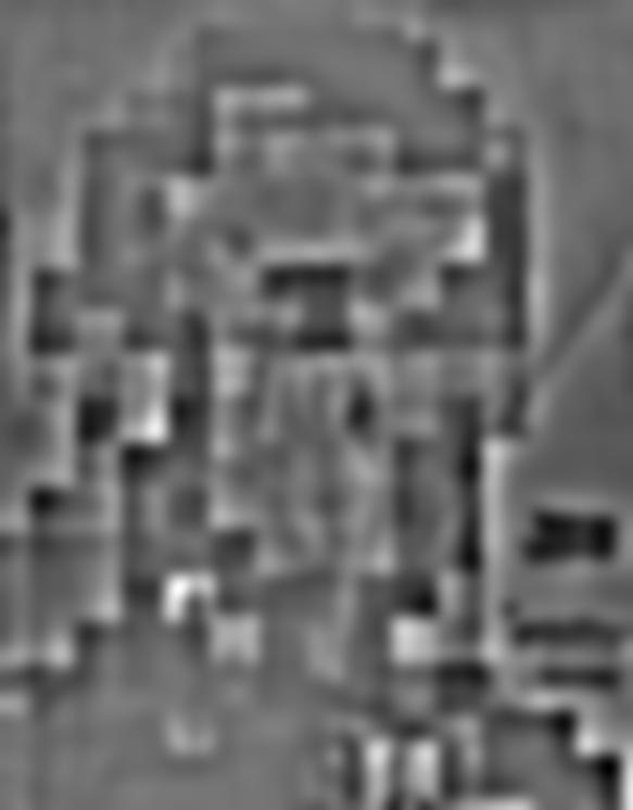
FFT of christian_bale.jpg |
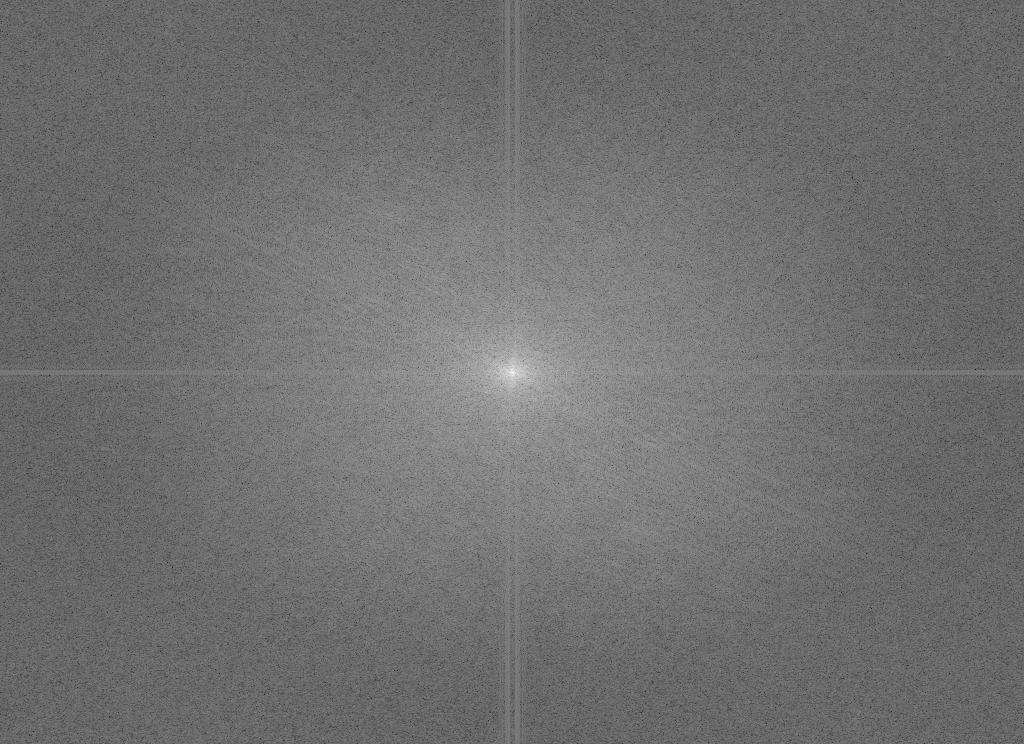
FFT of joker.jpg |
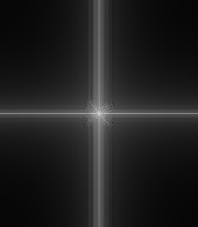
FFT of the lowpass filtered christian_bale.jpg |
FFT of the highpass filtered joker.jpg |
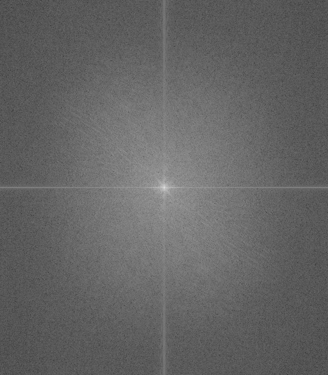
FFT of the hybrid christian_joker.jpg |
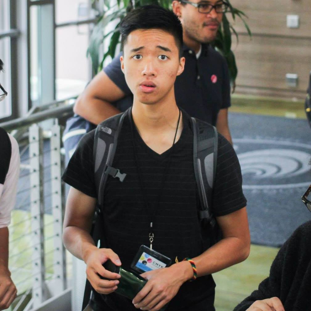
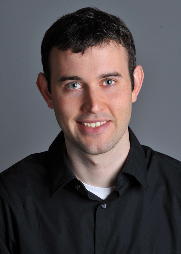
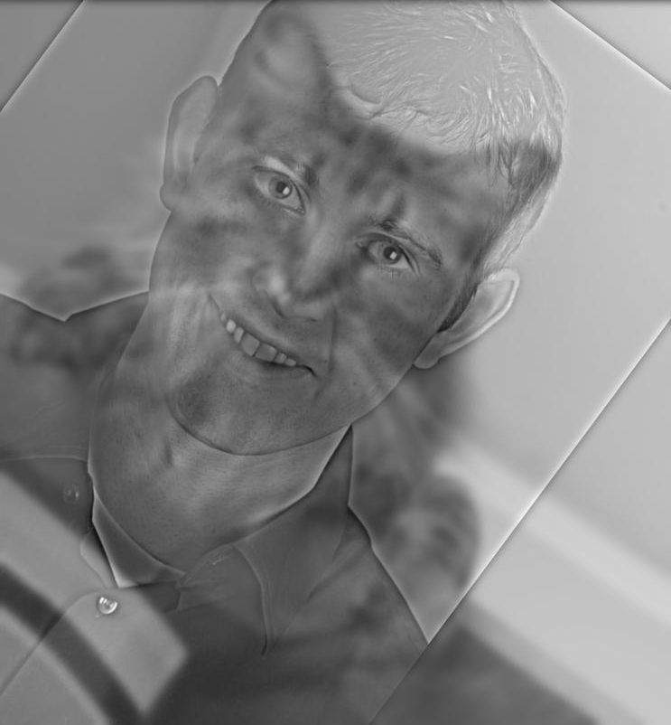
jacob.jpg |
+ |
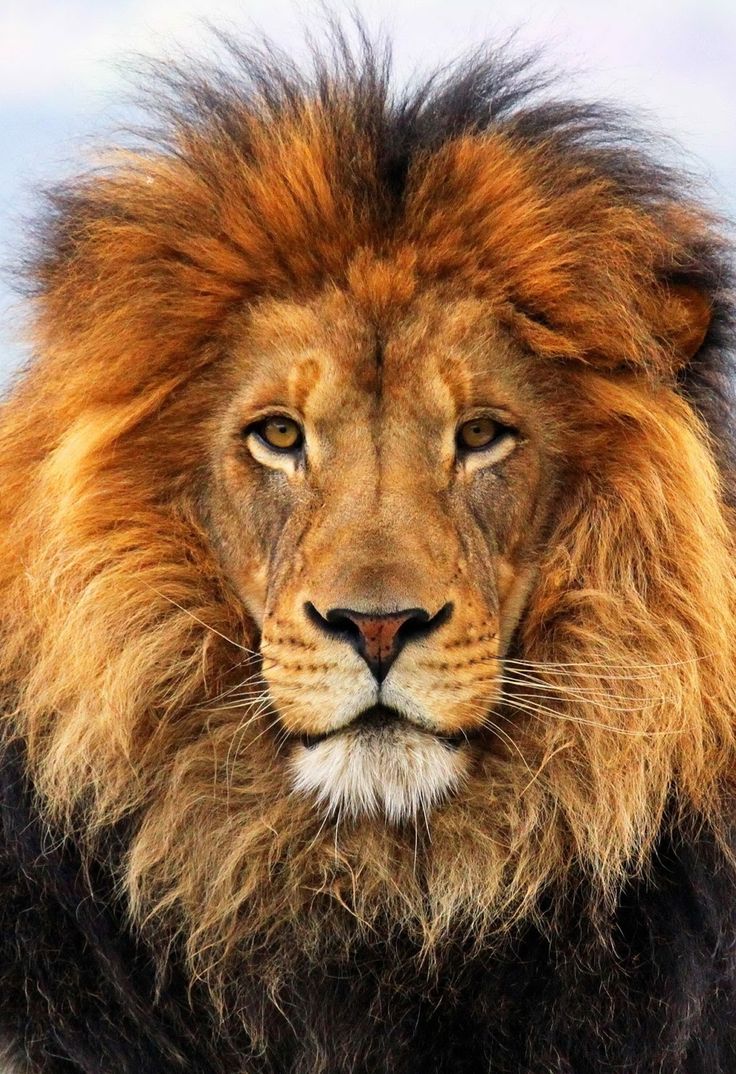
lion.jpg |
= |
jacob_lion.jpg |
Part 1.3: Guassian and Laplacian Stacks
Approach
The idea behind creating a Gaussian and Laplacian stack is relatively straightforward. Instead of downsampling the image repeatedly to create a Gaussian pyramid, we simply apply a Gaussian filter to the same image multiple times with different sigma values. The different sigma values determine the amount of blur that is created, giving us different samples of a single image. Constructing a Laplacian stack involves subtracting the i+1th Gaussian stack layer with the ith Guassian stack layer to create the ith Laplacian layer. Notably, in order to create the nth Laplacian layer, we must compute an additional n+1th Gaussian layer. The Gaussian stack generated has an ascending sigma value of sigma = 2i where i is the layer of the current stack, starting at 0.

|
| Gaussian Stack |

|

|
|

|

|
| Laplacian Stack |
|
|
|
|
|
|
| Gaussian Stack |

|

|

|

|

|
| Laplacian Stack |
|
|
|
|
|
|
| Gaussian Stack |

|

|

|
|

|
| Laplacian Stack |
|

|
|
|
|
Part 1.4: Multiresolution Blending
Approach
Multiresolution blending involves the two images we would like to blend together and a mask. A mask is simply a bit field where the pixel intensity of some pixels is zero and for others non-zero. Wherever the pixel intensity is zero in the mask, the pixel intensity of the masked image will be set in the background. Wherever the pixel intensity is non-zero in the mask, the pixel intensity of the masked image will be set in the foreground. What this allows us to do is to choose the location of where the two images will be blended. The first step to creating a multiresolution blend involves creating Laplacian stacks of the two images to be blended. We can create the Laplacian stack of each image by following the steps provided in the previous section. Let's call the Laplacian stack of the first image LA and the Laplacian stack of the second image LB. Next, we create a Guassian stack of the mask. Let's call this resulting Gaussian stack GR. We then flatten the two Laplacian stacks and the Gaussian stack together, weaving the layers of each stack with the following formula: LS[i] = GR[i] * LA[i] + (1 - GR[i]) * LB[i] where i is the ith layer of the stack.

apple.jpg |
+ |

orange.jpg |
+ |

oraple_mask.jpg |
= |
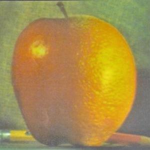
oraple.jpg |
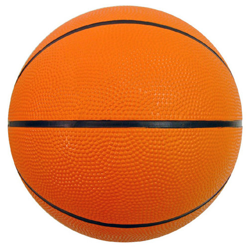
basketball.jpg |
+ |
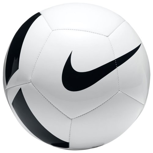
soccer.jpg |
+ |

basketsoccer_mask.jpg |
= |
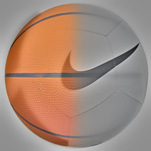
basketsoccer.jpg |
kid.jpg |
+ |
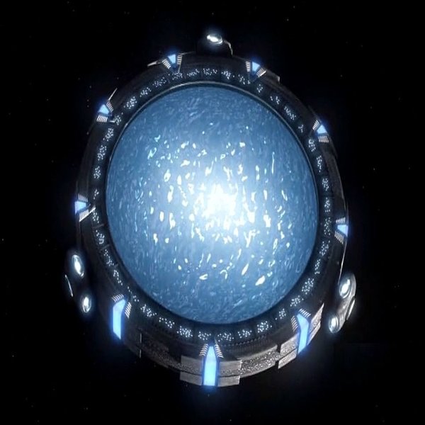
stargate.jpg |
+ |
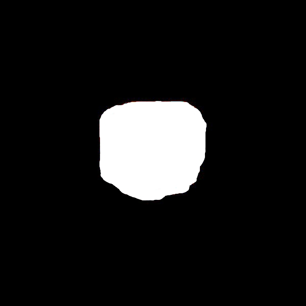
kidgate_mask.jpg |
= |
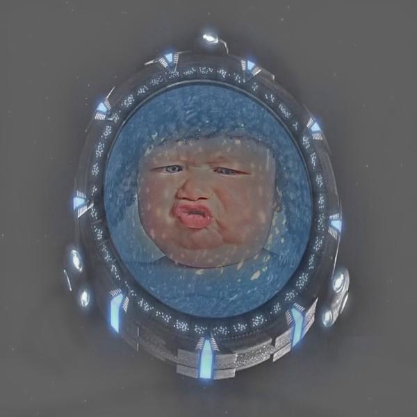
kidgate.jpg |
Part 2.1: Toy Problem
Approach
In this problem, we are tasked to recreate an image using the image's x and y gradients. To do so, we create a sparse matrix with dimensions (((m-1)*n + (n-1)*m + 1, m*n) where m and n are the height and width of the original image, respectively. The (m-1)*n term denotes the amount of y-gradients we are sampling from the image, the (n-1)*m denotes the amount of x-gradients we are sampling from the image and the +1 term is for the top-left corner of the image.
toy_problem.png |

toy_problem_gradient.png |
Part 2.2: Poisson Blending
Approach
The blends of the previous approaches had extremely noticeable seams at the border of the images. In order to create seamless blends, we can use Poisson blending. We can do this by aligning the images using the given MATLAB starter code, generating a mask, and populating a sparse matrix as detailed in the previous section. The main difference in the approach of this part and the approach of the previous part is the amount of gradients we are doing. In the previous section, we only calculated the gradient of x and y in a single direction. In this part, we will calculate the gradient of x and y in both directions, resulting in 4 total gradients per pixel. Furthermore, we will only need to take the gradient of the source image at the pixels indicated by the mask. Any pixel outside of the mask will be simply copied over.
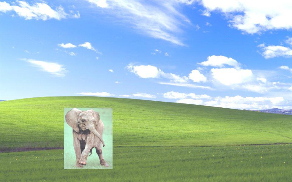
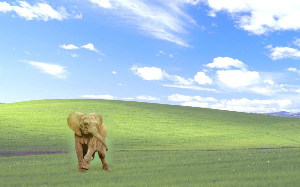
source.png |
target.jpg |

direct.jpg |
blend.jpg |
source.png |

target.jpg |
direct.jpg |

blend.jpg |
source.png |
target.jpg |
direct.jpg |
blend.jpg |
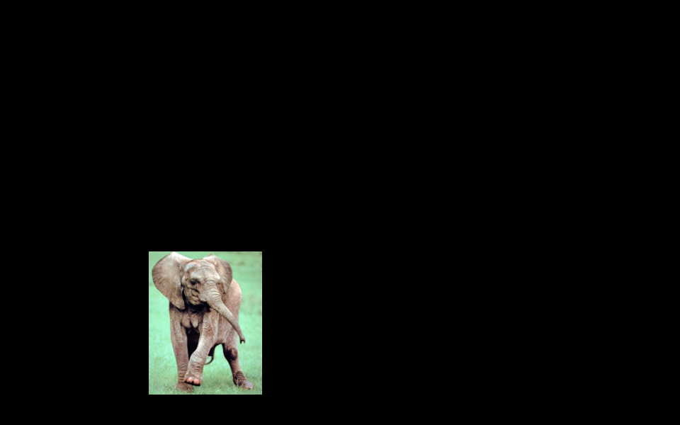
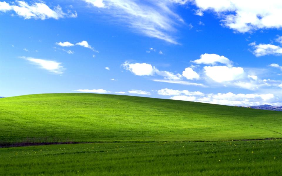
The main reason why this blending was so poor is because the background of the images are not similar enough to blend seamlessly. Even though the elephant is in a green background, the pixel intensity of the background of the elephant is much lower than the pixel intensity of the bliss image. The gradient of such differing background would be so large, outputting a poor blended image.

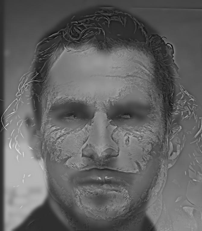
christian_bale.jpg |
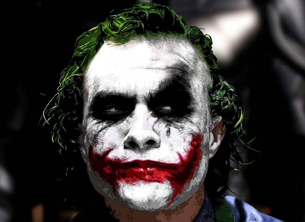
joker.jpg |

christian_joker.jpg |
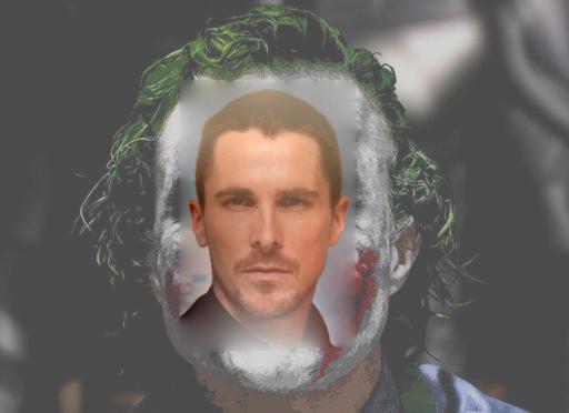
blend.jpg |
I used poisson blending to blend together Christian Bale and the Joker, which were the images I used to create a hybrid image in part 1. Clearly, poisson blending is much worse in this case. Poisson blending is best used when the background of both images are relatively similar. The reasoning behind this is because the gradient of two pixels that are similar is much more smooth than the gradient of two pixels with differing color and intensity. The method of separating low and high frequencies as in hybrid images ignore pixel intensity and deals with images in the fourier domain, therefore resulting in better hybrid images when the backgrounds of the two images are different.