CS194-26 Project 3: Gradient-Domain Fusion
By Kaiwen Zhou
Part 1: Frequency Domain
In the first part of this project, we play with different frequencies within images in order to perform certain post-processing tasks such as image sharpening, producing hybrid images, analyzing images using Gaussian and Laplacian stacks, and multiresolution blending of images.
1.1: Warmup (Sharpening)
For this part, I sharpened an image using the unsharp mask technique. I blurred an image by convolving it with an (11, 11) Gaussian blur kernel with a sigma of 3. From there, I obtained the unsharp mask by subtracting the blurred image from the original, and added those details back into the original image to sharpen the edges, scaled by an alpha of 3. The image came out slightly oversharpened.
Results
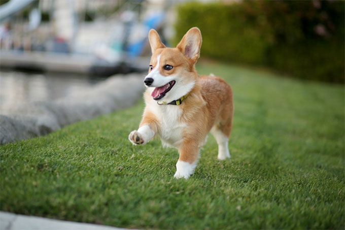 original image
|
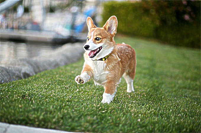 sharpened image
|
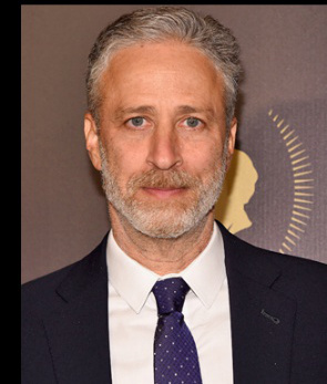
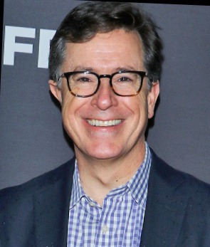
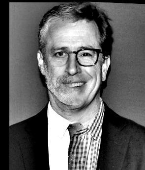
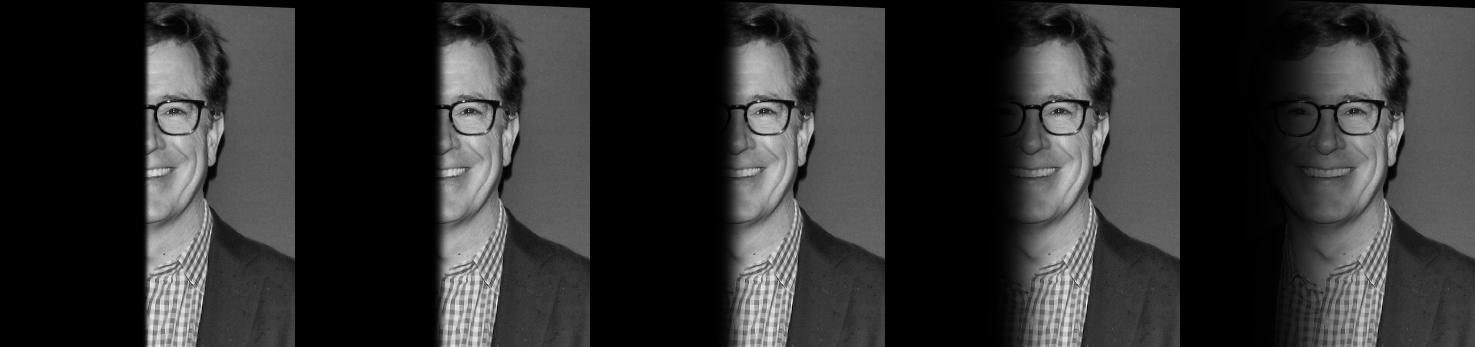
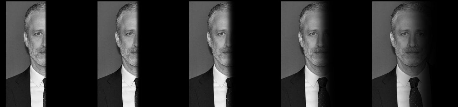
1.2: Hybrid Images
Overview
Hybrid images can be obtained by taking a low pass filtered image and a high pass filtered one, and then combining the two to form a single hybrid image.
Favorite
|
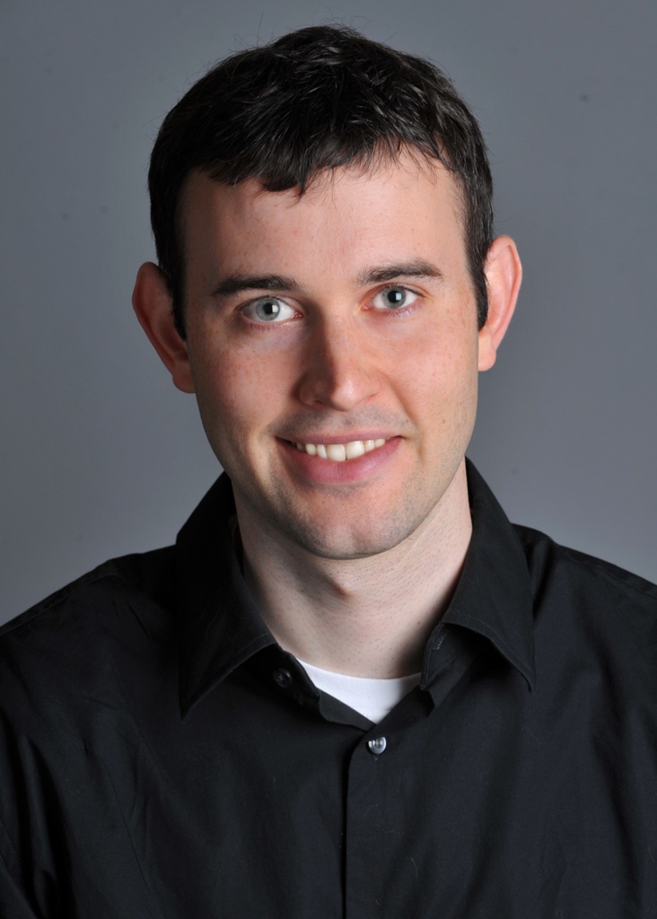
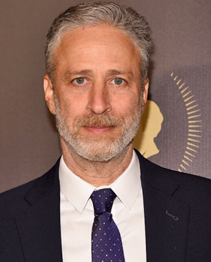 jon
jon
|
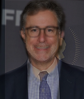
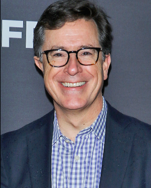 stephen
|
 hybrid jon stephen
|
Below, I used skimage.exposure.equalize_hist to equalize the FFT images in order to make them more visible.
FFT Analysis
|
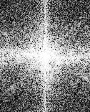 stephen fft
|
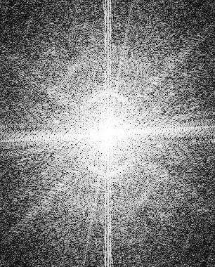 jon fft
|
|
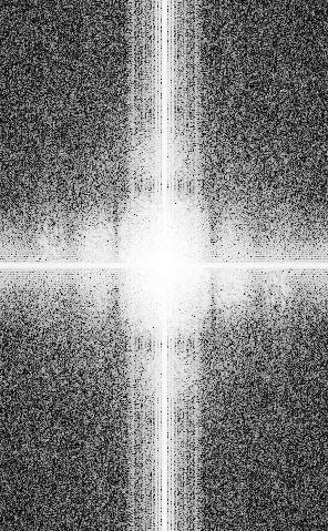 low pass (stephen) fft
|
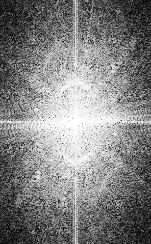 high pass (jon) fft
|
|
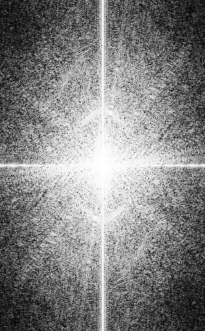 hybrid fft
|
Other Example
|
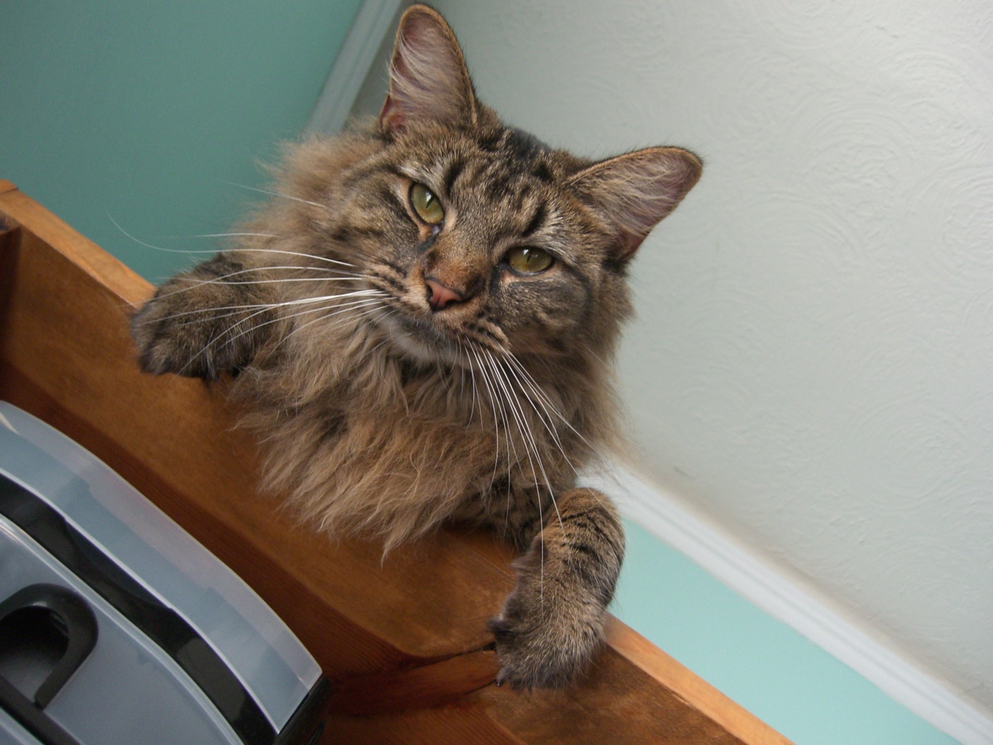 cat
cat
|
 derek
derek
|
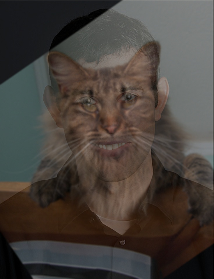 hybrid derek cat
|
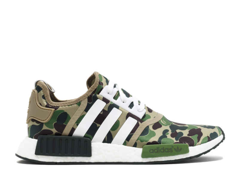
Failure Case
|
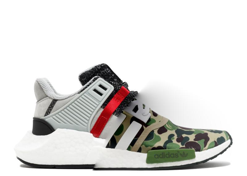
 bape
bape
|
 overkill
|
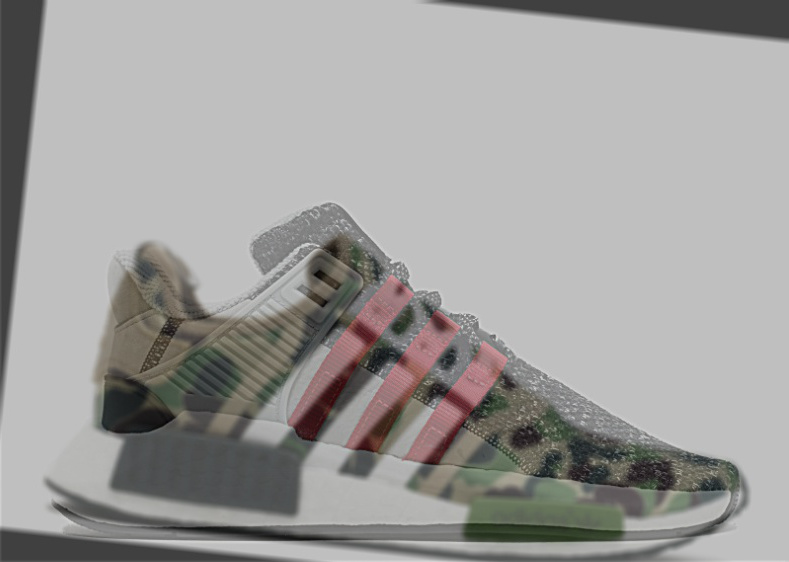 hybrid overkill bape
|
I wanted to hybridize the images of these two shoes together, but the resulting image doesn't look good. The pattern on the Bape shoes stands out too much compared to that of the Overkill shoes, so the image just looks like an overlay.
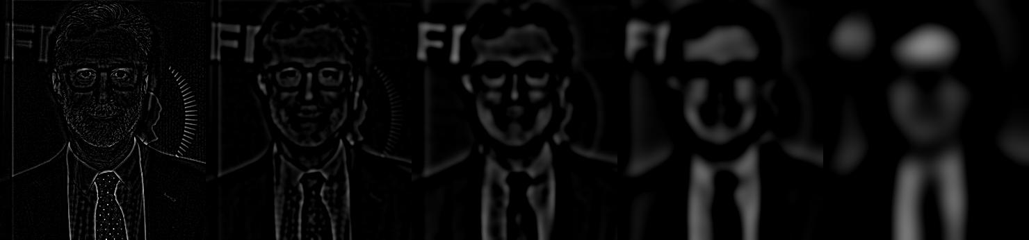
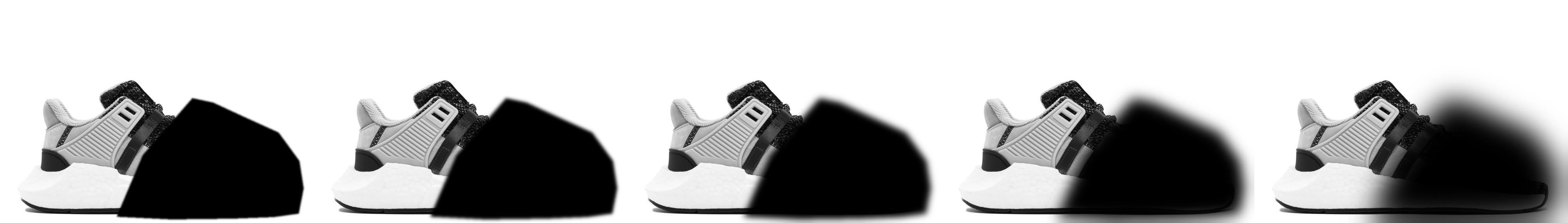
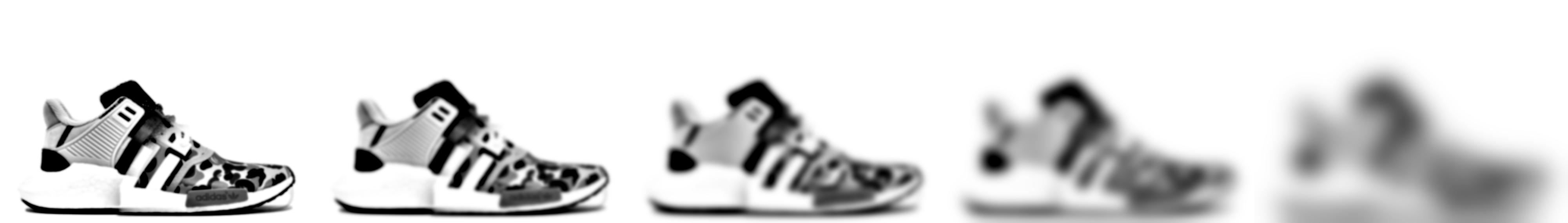
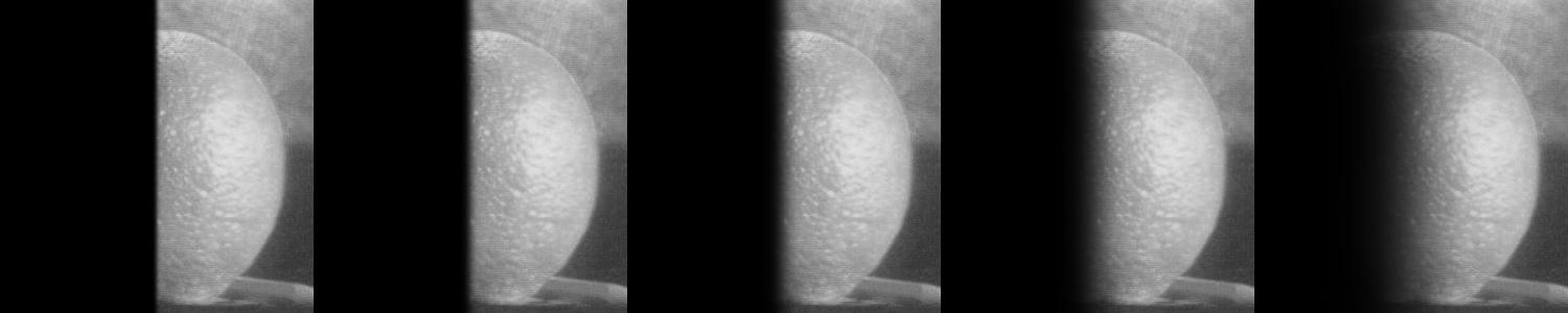
1.3: Gaussian and Laplacian Stacks
Overview
Using Gaussian and Laplacian stacks, we can analyze images that contain structure at different resolutions. The Gaussian stack shows different levels of Gaussian blurring (low-pass filtering) for the image, with the sigma used at each level of the stack doubled at each subsequent level. Meanwhile, the Laplacian stack is constructed out of the differences of blurred images between each consecutive level of the Gaussian stack.
My implementation uses a Gaussian kernel of size 45 and builds stacks that are 5 levels deep. The first level of the Gaussian stack uses a sigma value of 2, and doubles at each subsequent level.
For my results, I chose to analyze the canonical exampe of Lincoln's Dali in addition to my Jon-Stephen hybrid image.
Results
|
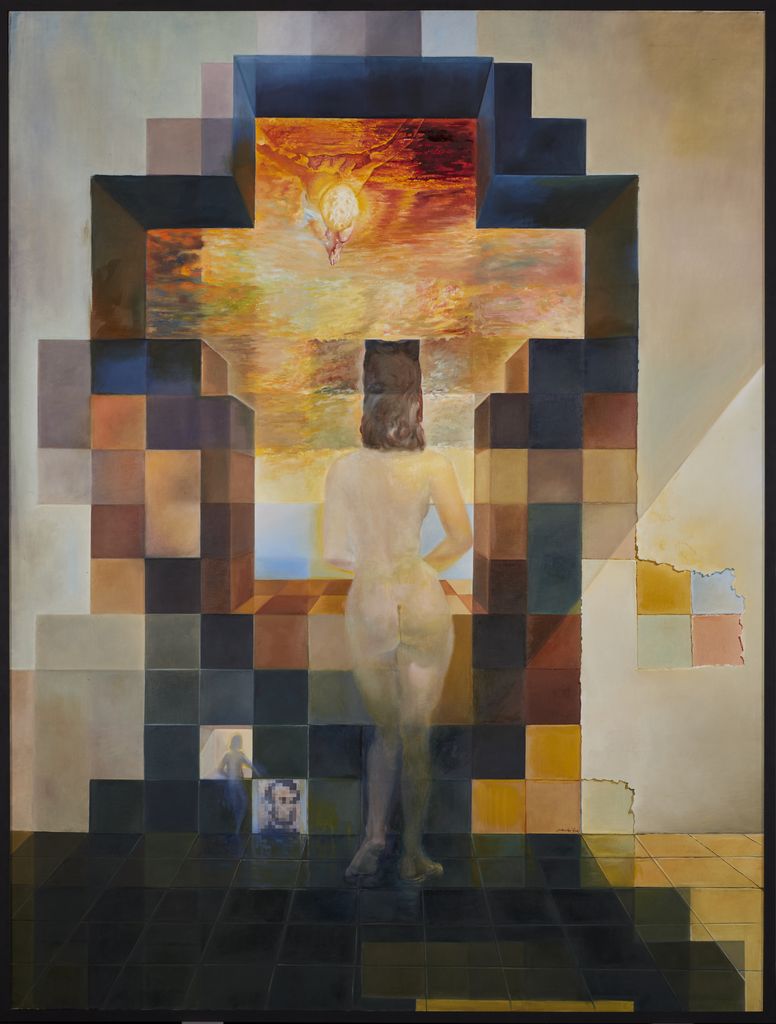 lincoln dalivision
|
|
|
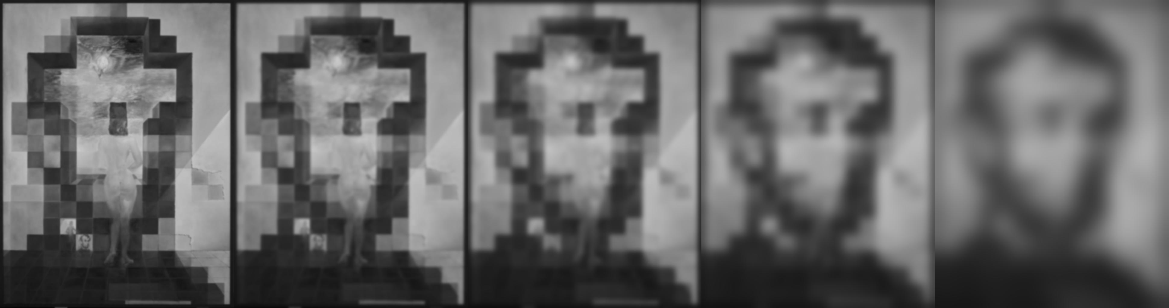 lincoln gaussian stack
|
|
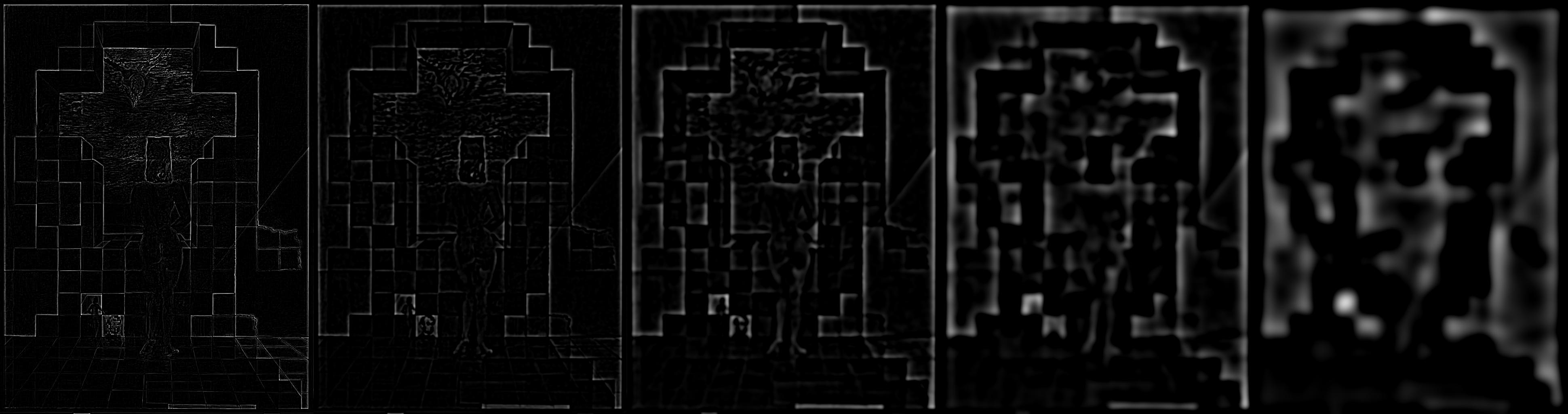 lincoln laplacian stack
|
|
 stephen jon hybrid
|
|
|
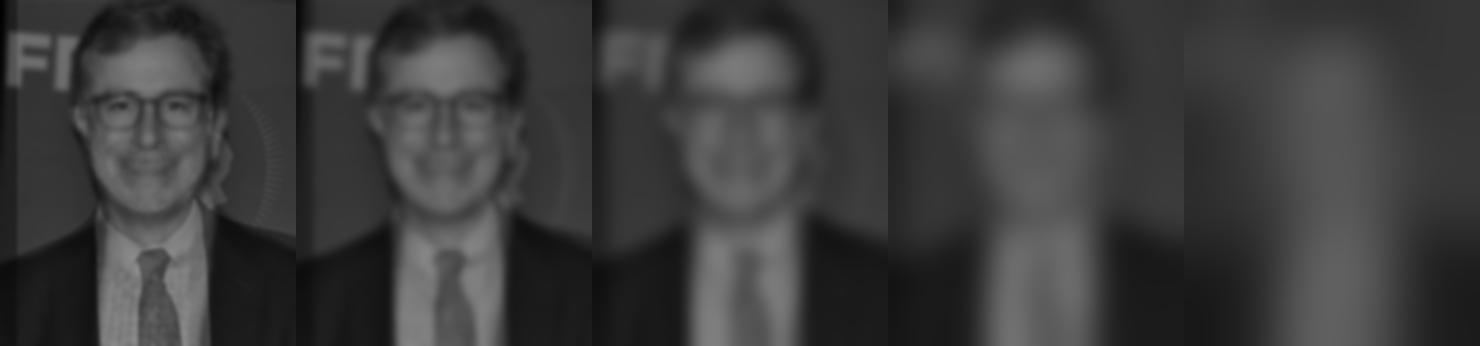 jephen gaussian stack
|
|
 jephen laplacian stack
|
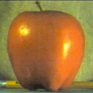
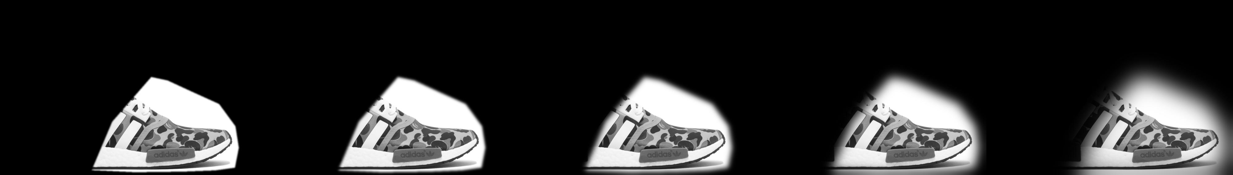
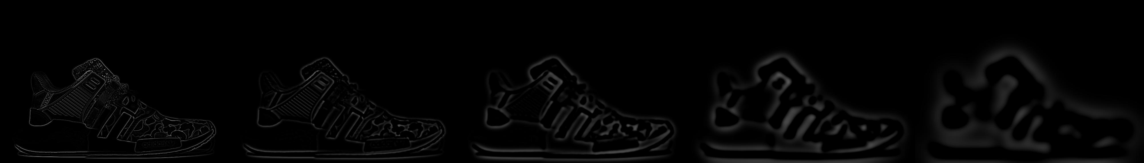
1.4: Multiresolution Blending
In this part, we perform multiresolution blending to produce a gentle seam between two images separately at each band of image frequencies. This results in a much smoother seam that gently blurs one image into another.
To do this, we perform the blending operation by producing a Laplacian stack for the image and a Gaussian stack for the mask being used. Here, the mask represents the region of the image that will be splined into the other image. Thus, we have two Laplacian stacks and one shared Gaussian stack for the mask. Using these three stacks, we blend the two corresponding channels together by weighting each channel's contribution in the new image based on where they fall in the current level of Gaussian stack.
My implementation uses 5 levels for the Gaussian and Laplacian stacks, builds its Gaussian stacks starting at a sigma value of 2 and doubling at each subsequent level, and uses a Gaussian kernel of size 45.
Favorite
|
 bape
bape
|
 overkill
|
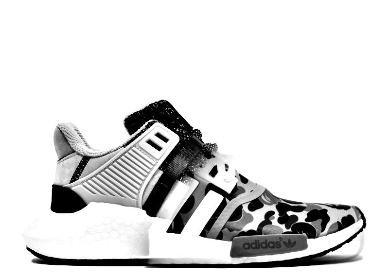 overkill-bape hybrid
|
|
 bape gaussian
|
|
 overkill gaussian
|
|
 blend gaussian
|
|
 blend gaussian
|
Other results
|
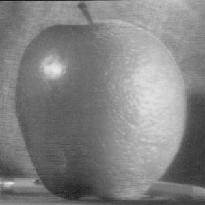
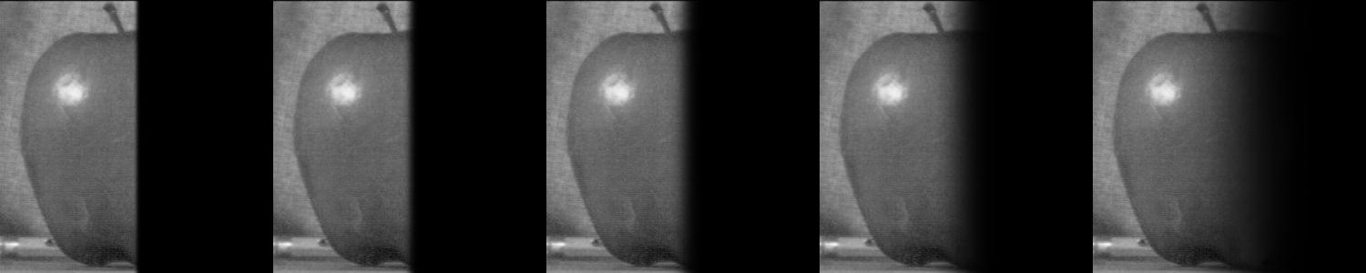 apple gaussian
|
|
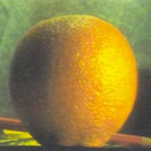
 orange gaussian
|
|
 jon gaussian
|
|
 stephen gaussian
|
Part 2: Gradient Domain
In this part, we explore gradient-domain processing and apply it to seamlessly blend an object from a source image into a target image.
The easiest way to do this is to simply copy and paste a region of pixels from the source image directly into a target location in the target image. However, this method usually results in very noticeable seams. Instead, because human perception tends to be more sensitive to gradients than absolute intensity values, we attempt to smooth seams by solving for new target pixel values that maximally preserve the gradients present in both our target and source images. As a side effect, our blending may cause discolorations in intensity values, but will have smoother gradients and thus will be more visually appealing.
Below, we explore Poisson Blending.
2.1: Toy Problem
Overview
Before blending images using the Poisson blending method, we first tackle the simpler problem of reconstructing an image s from only its gradients and one pixel value.
 original image
|
 reconstructed image
|
2.2: Poisson Blending
Overview
We now proceed to implement the Poisson blending method. The inputs to the method are (1) a source image, (2) a target image, and (3) a binary mask whose white pixels specify regions to be blended. We construct a matrix equation Av = b, where v is the final blended image that we desire. A and b are defined such that for each pixel (i, j) within our mask, b(i,j) is the sum of differences between (i, j) and all four neighboring pixels (Laplacian kernel). A is a sparse matrix similarly defined with the Laplacian kernel within our mask, so that v(i,j) has a similar constraint to that of b. Outside of our mask, b(i,j) is simply the target pixel, and A(i,j) is simply 1.
For our implementation, we require that the source and target images, as well as the mask image, all have the same size. Since they all have the same size, the source regions and target regions occupy the same pixel indices and can therefore be specified by the same mask image. We use the provided Matlab starter code to align the images and construct the masks, as pictured below.
Results
 gabe original image
|
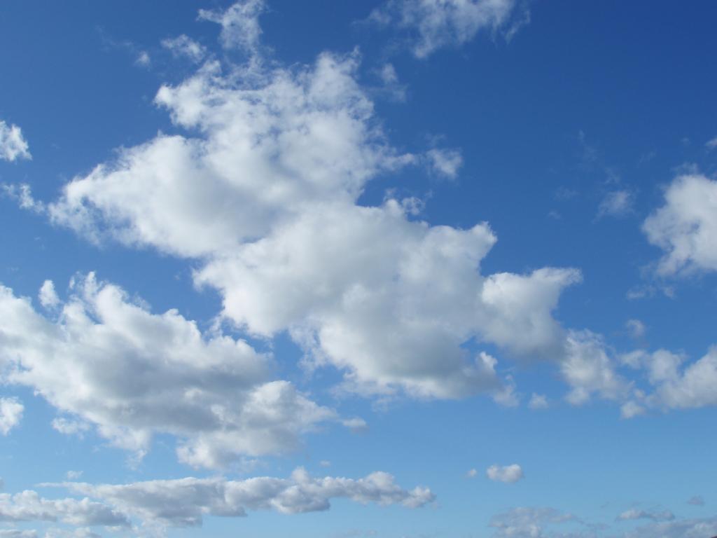 background image
|
|
 gabe aligned image
|
 gabe mask
|
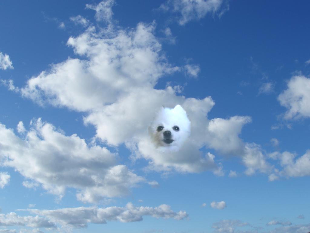 gabe blended with cloud background
|
|
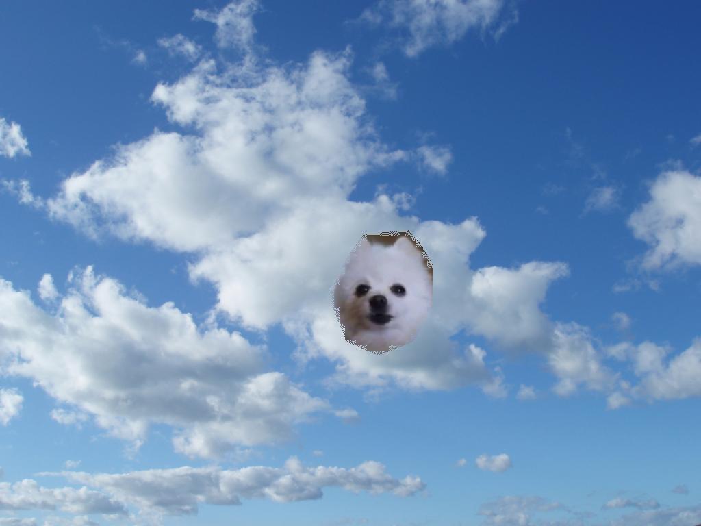 gabe copied onto cloud background
|
Other examples
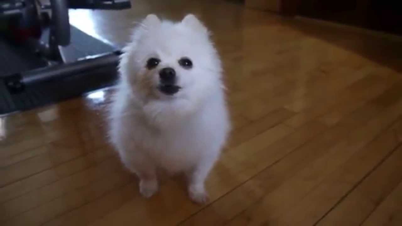
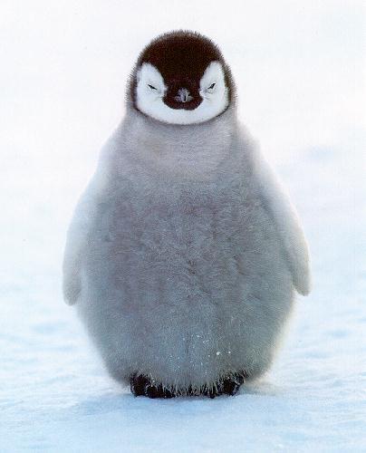 penguin original image
|
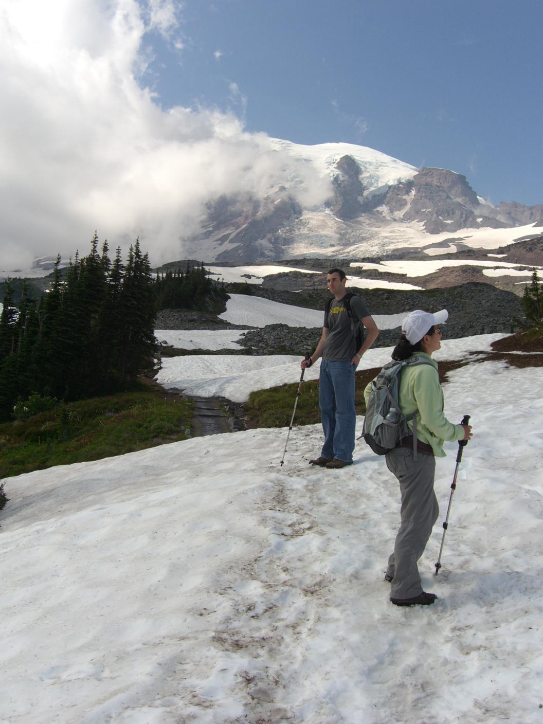 background image
|
|
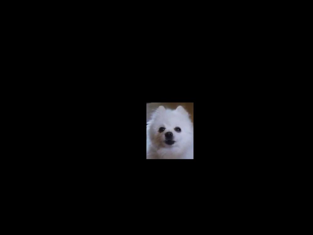
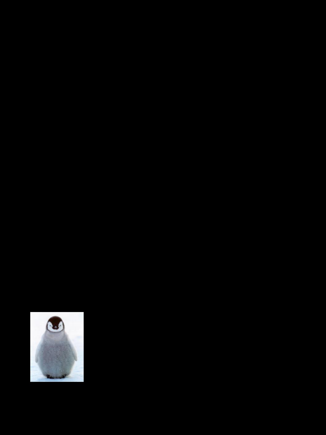 penguin aligned image
|
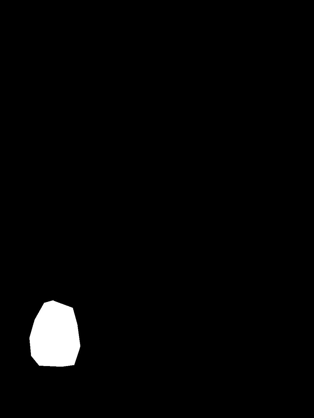 penguin mask
|
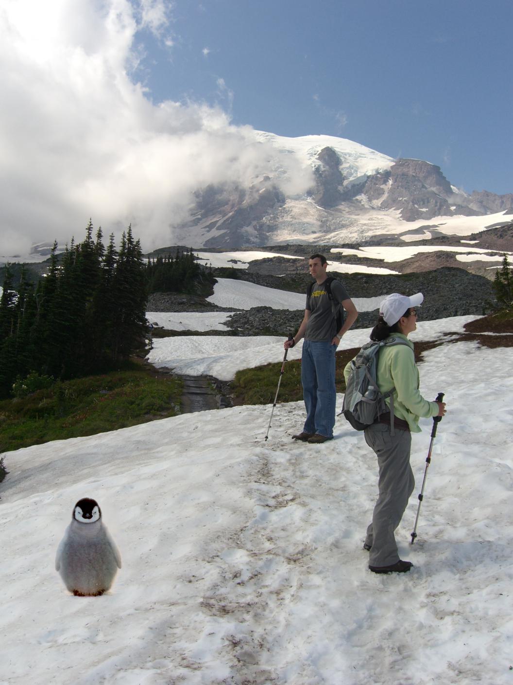 penguin blended with background
|
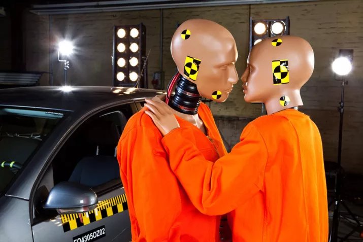 dummy original image
|
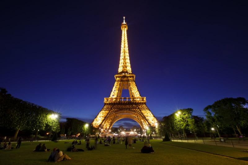 background image
|
|
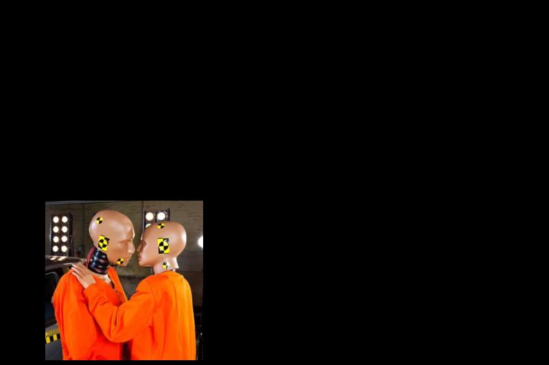 dummy aligned image
|
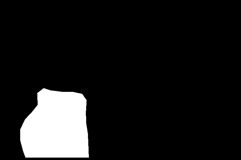 dummy mask
|
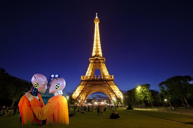 dummy blended with tower background
|
Failure example
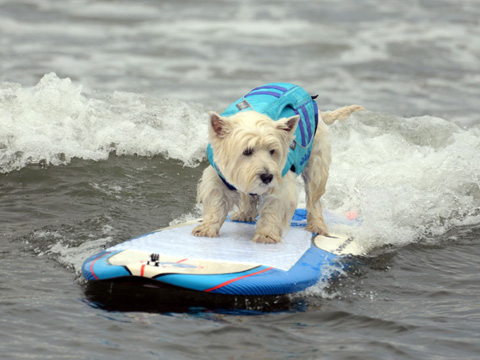 surf original image
|
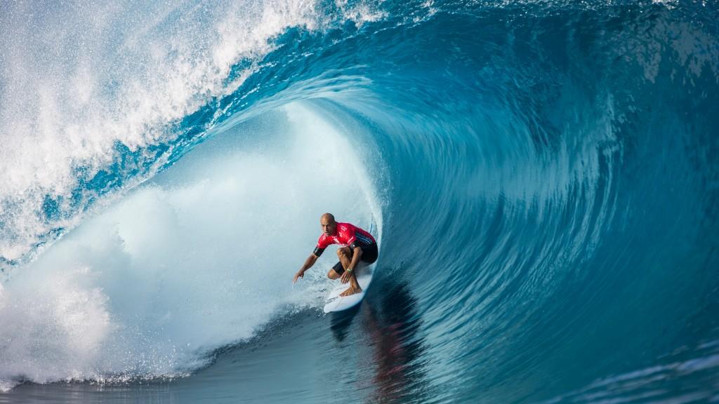 background image
|
|
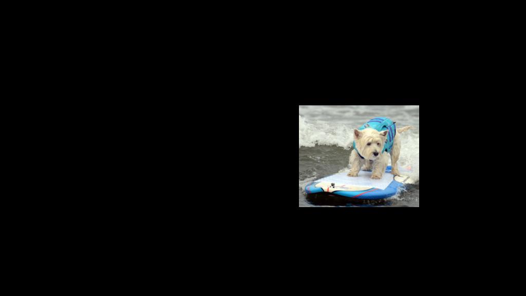 surf aligned image
|
 surf mask
|
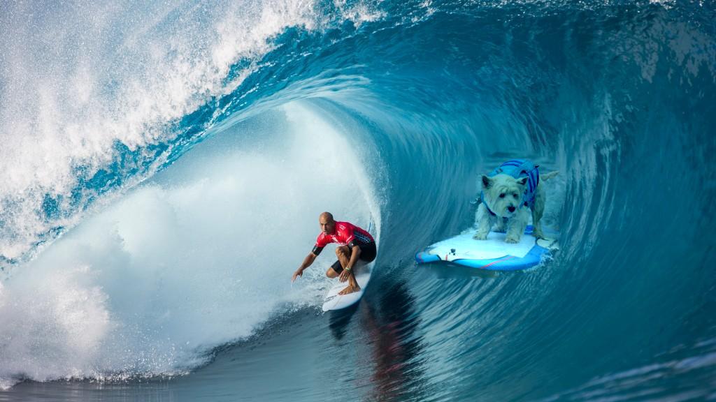 surf blended with wave background
|
Our blending looks off. Because I blended the dog into the middle of the wave, the dog was colored with the intensities of the wave, giving it an unnatural bluish tinge.
Comparison of blending functions
|
bape
|
overkill
|
|
Multiresolution blending
|
 Poisson blending
|
Comparing multiresolution blending and poisson blending, multiresolution blending seems more appropriate for this sort of image. Poisson blending seems most appropriate for integrating an image into a single-intensity background, while multiresolution blending seems to work better for seamless blending of contrasting textures, such as this combination of two different shoes.