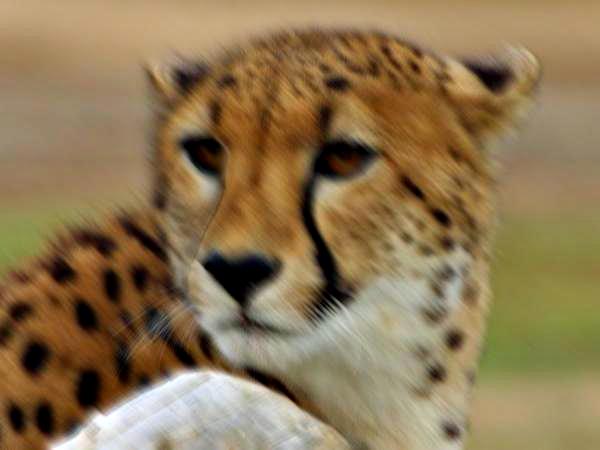
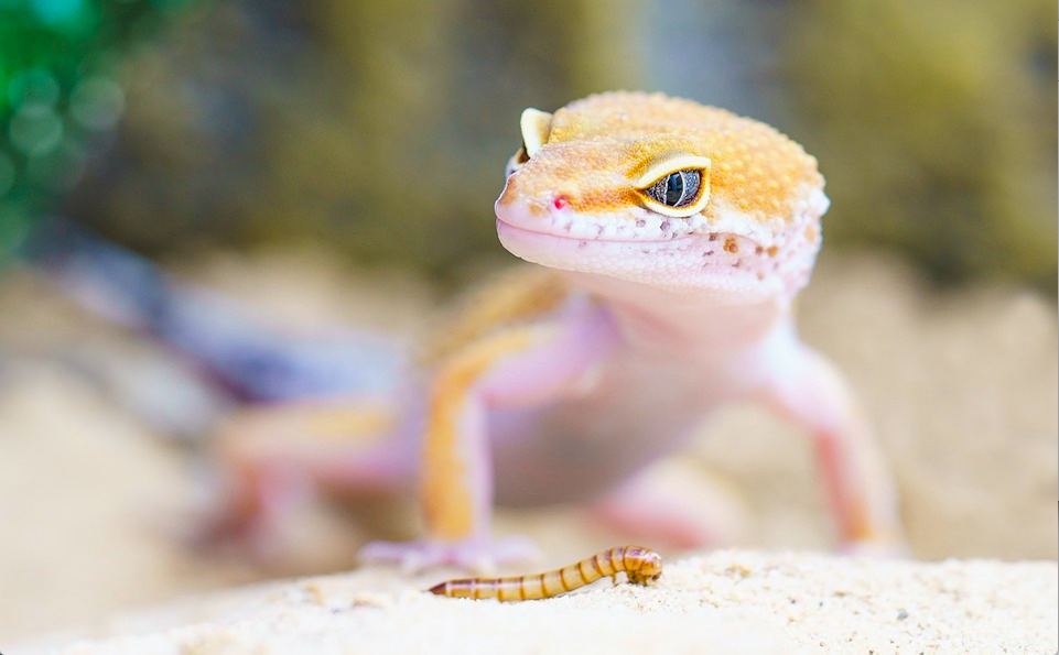
Part 1.1: Warmup For this portion of the assignment, the goal was to sharpen a blurry image. I found a blurry image of a leopard online, ran a high pass filter on the image (subtracted the gaussian from the original image), and added an alpha factor of the laplacian to the original image. The results are shown below. (Blurred, Sharpened)
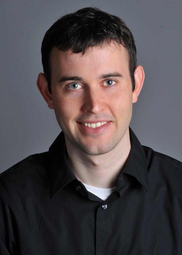
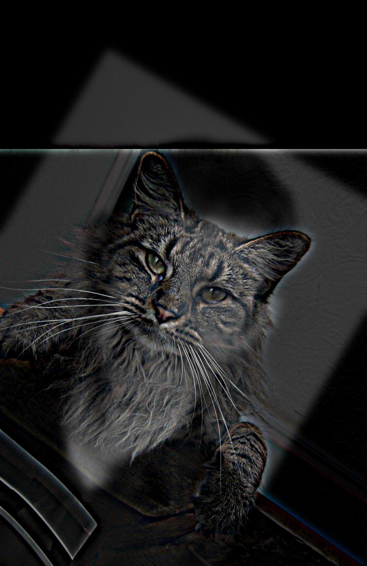
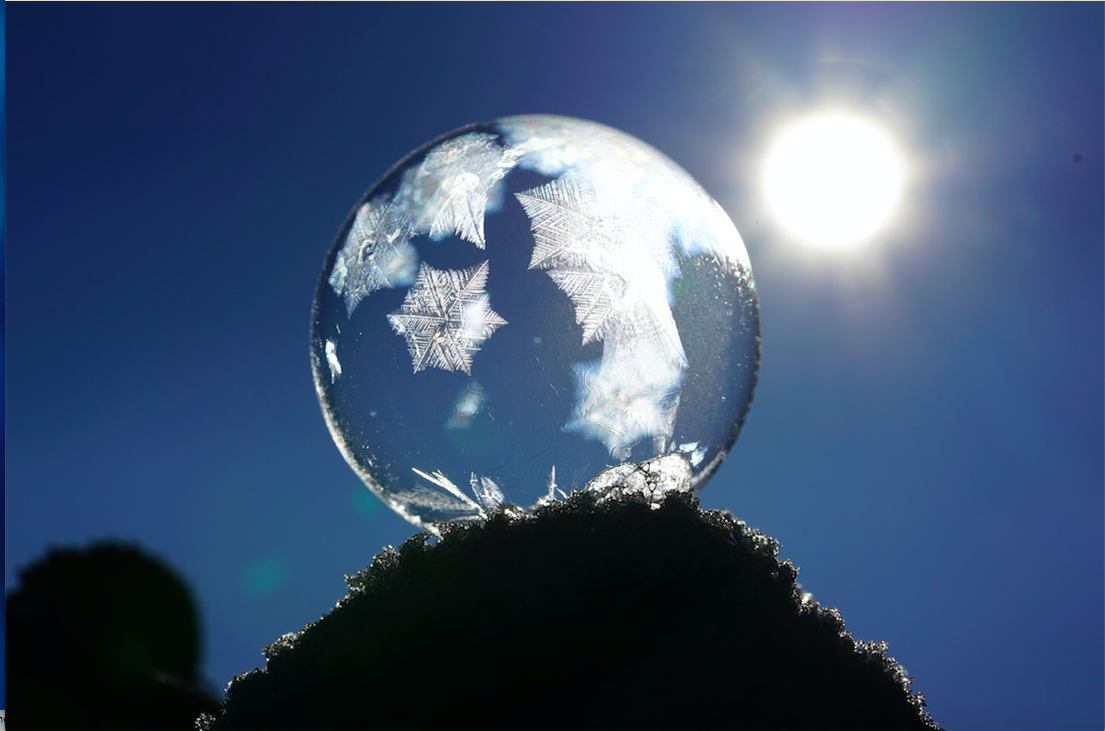
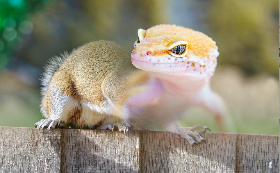
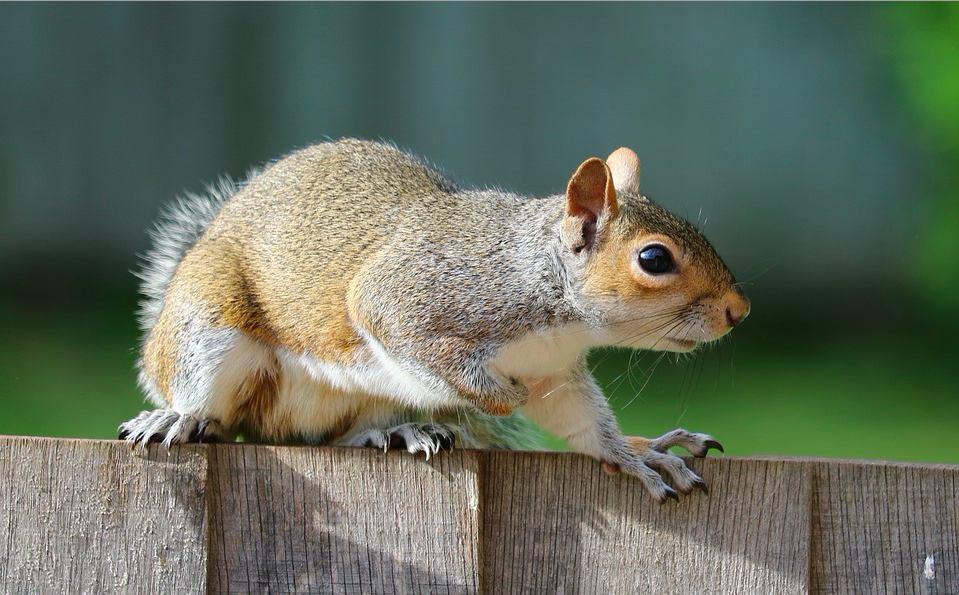
Part 1.2: Hybrid Images For the next portion of the assignment, the goal was to disguise two images in a single one, by making use of the high and low frequencies that make up the images. This was accomplished by running a high pass filter on one image, and a low pass filter on the other, and then averaging the pixel intensities of the two filtered images at each pixel. The image onto which the low pass filter was applied was also converted into a grey image, as the color details did not help distinguish it from the other image. This was because color added extra noise that made the high-pass image difficult to distinguish up close (Which is also why color had a positive effect when left on the high-pass image, it added more details up-close that vanished at large distances). Below is the picture of Derek and the cat before and after running the program.
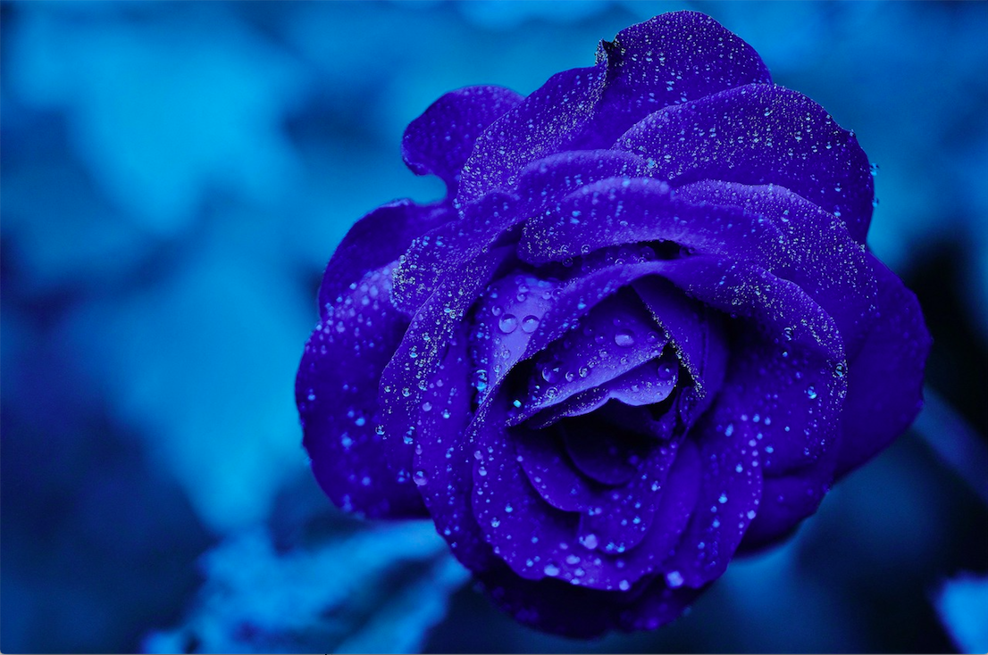
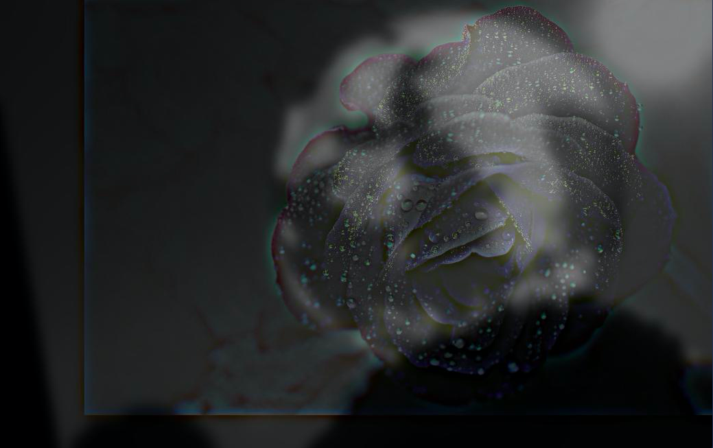
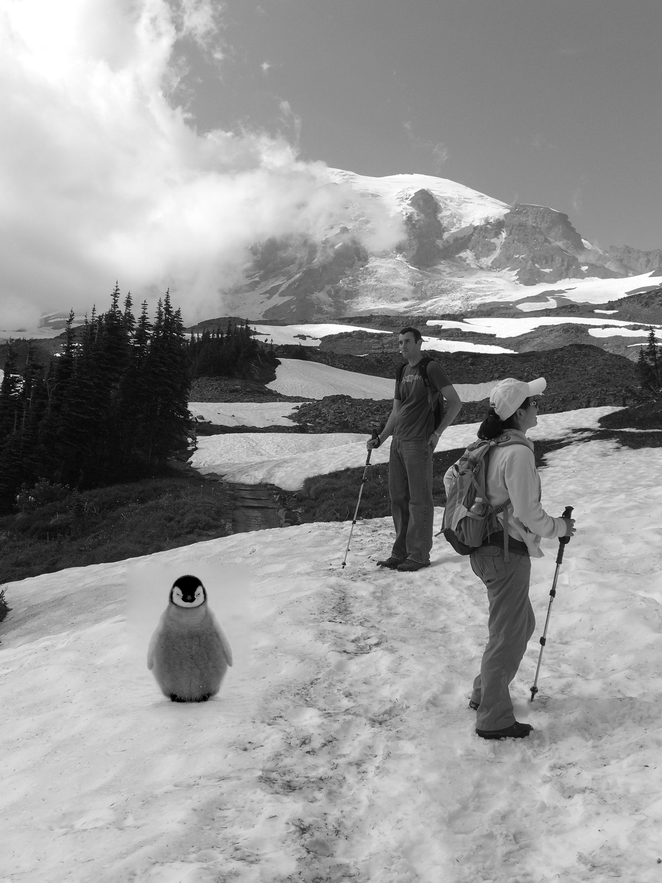
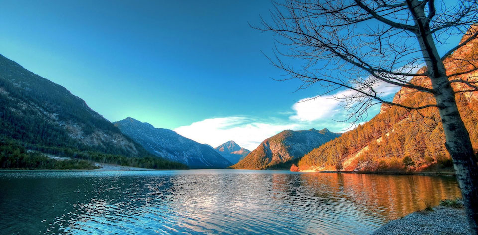
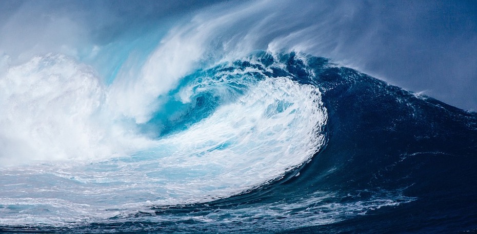
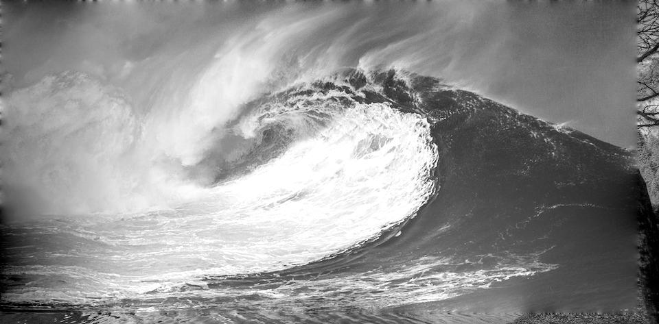
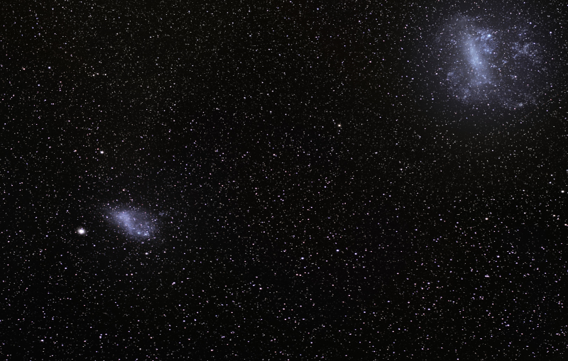
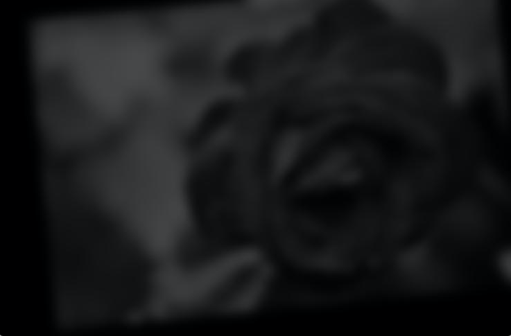
Finally, one particularly bad example occurs when using an image without many distinctive features/edges as the high-pass image. The flower image was used once again, but this time with a space picture blended in:
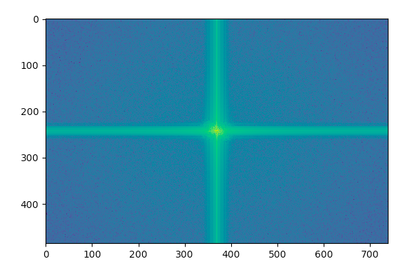
Part 1.3: Gaussian/Laplacian Stacks For this portion of the assignment, I recursively created a gaussian and laplacian stack, by recursively applying a gaussian filter to the image, computing the laplacian of the image, and then setting the new image to the gaussian. At the base level, the previously calculated gaussian was returned.
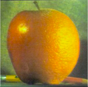
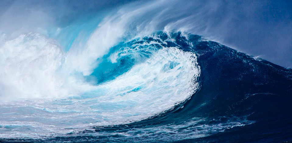
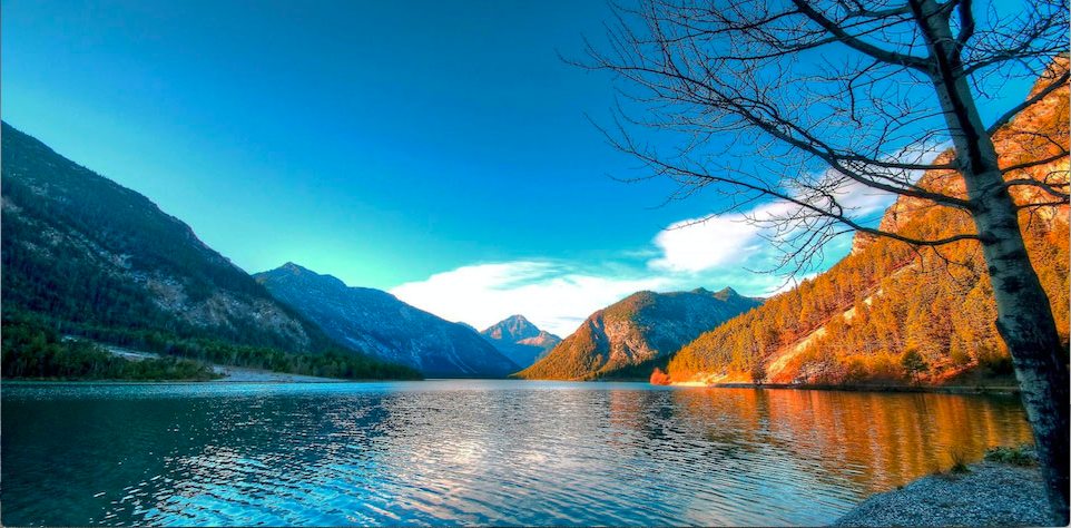
Part 1.4: Multiresolution Blending The goal of this portion was to blend two images together using a mask, which a gaussian filter was then applied to. This gradually reduces the pixel intensities near the edge of the mask, which allows another image (masked in the same way) to be overlayed on top, giving a smooth transition from the pixels of one image to the pixels of another. Using the color of the pixels as part of the gaussian filter improved the transition. A blend of the apple and orange can be seen below.
Part 2.1: A Toy Example For the first part of the poisson blending assignment, I formulate three different objectives, namely that: 1. The gradients of x-neighbors of each pixel match those of the source image as closely as possible 2. The gradients of y-neighbors of each pixel match those of the source image as closely as possible 3. The first pixel of the resulting image should have the same intensity as the first pixel of the source image This can be solved using a least squares solver, returning the original image.
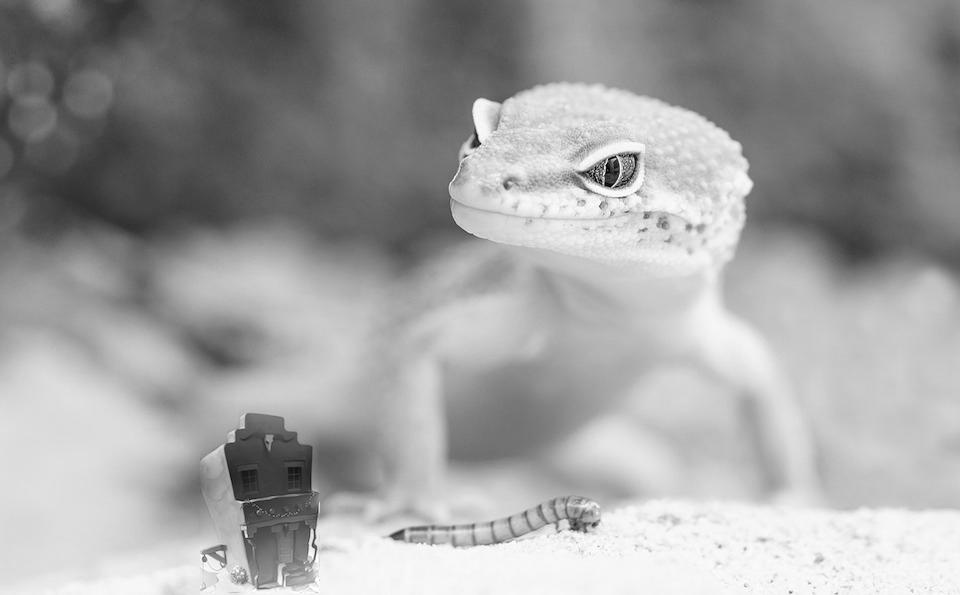
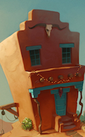
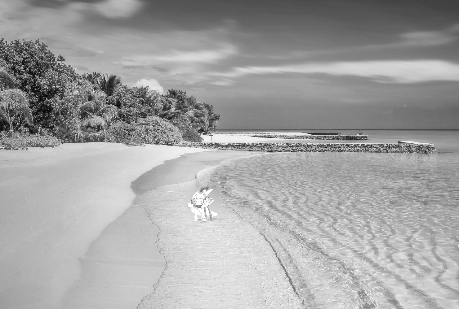
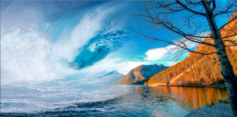
Part 2.2: A Toy Example For the final part of this assignment, the objective is to blend one image into another. Since I did not have matlab installed on my machine, I aligned the images and masked them manually. The only difference between this and part 1 is that now, I find the closed-form solution to the matrix. This requires a square matrix, so all the neighbors are compared as part of a single equation (and thus row in the matrix). Moreover, both the neighbors are compared in all directions, instead of just one direction as in 1. Finally, the edges of the image now consider the pixel intensities of the target image.