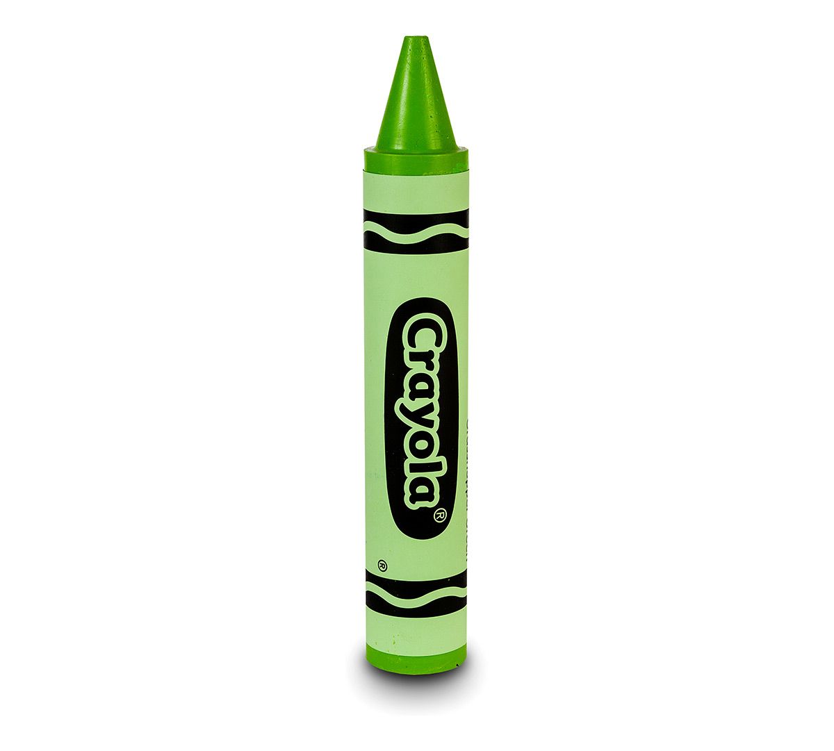
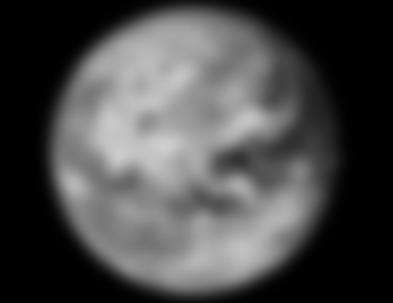
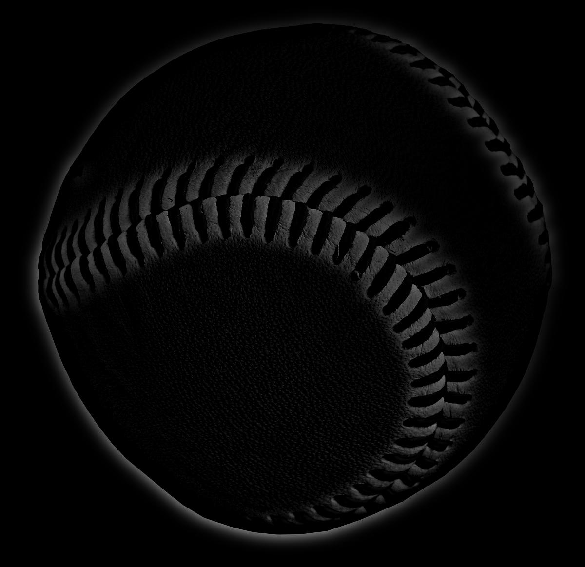
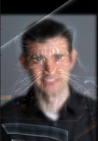
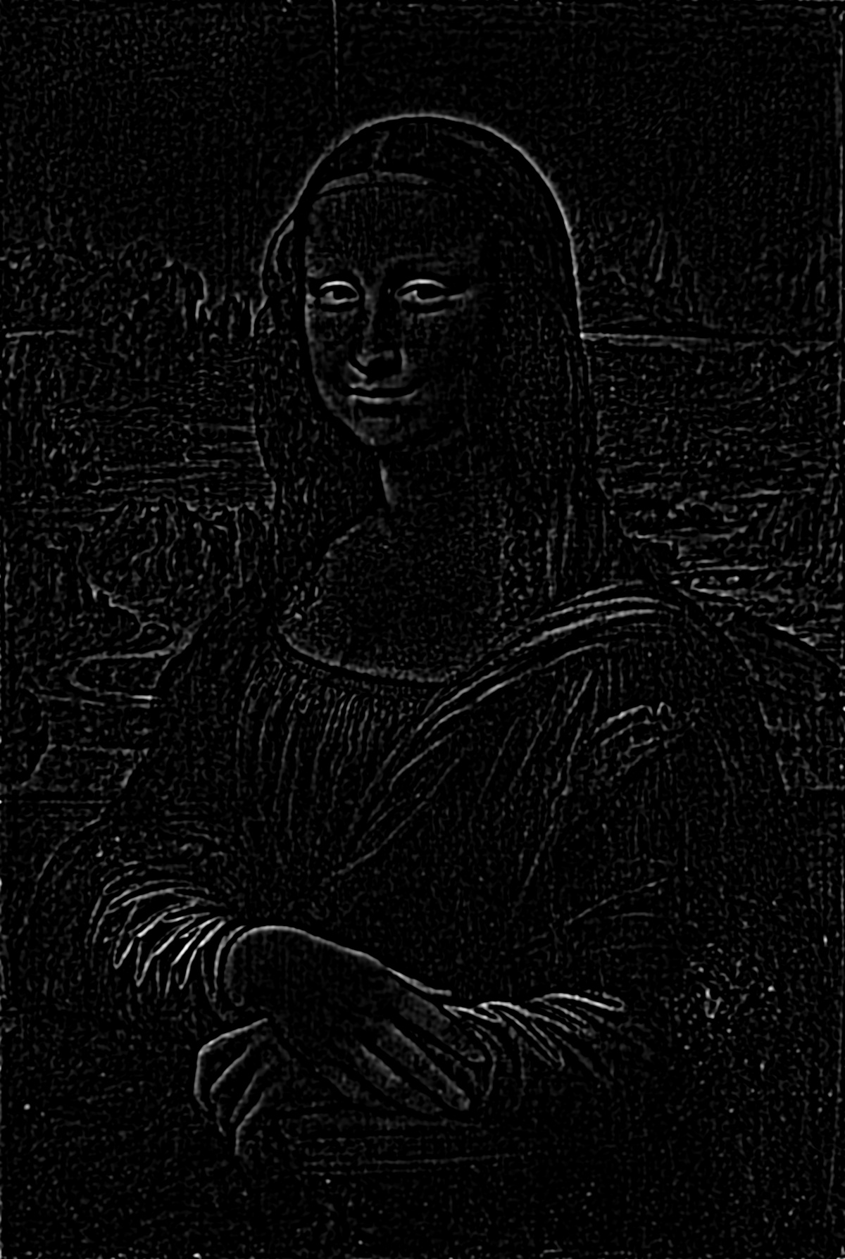
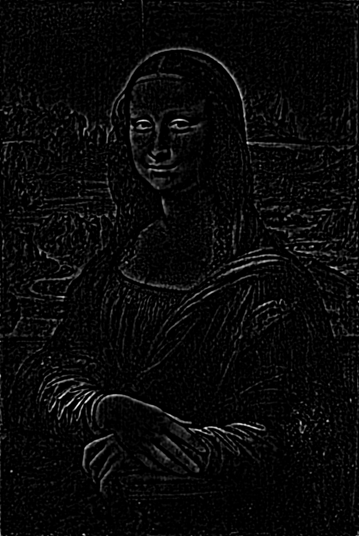
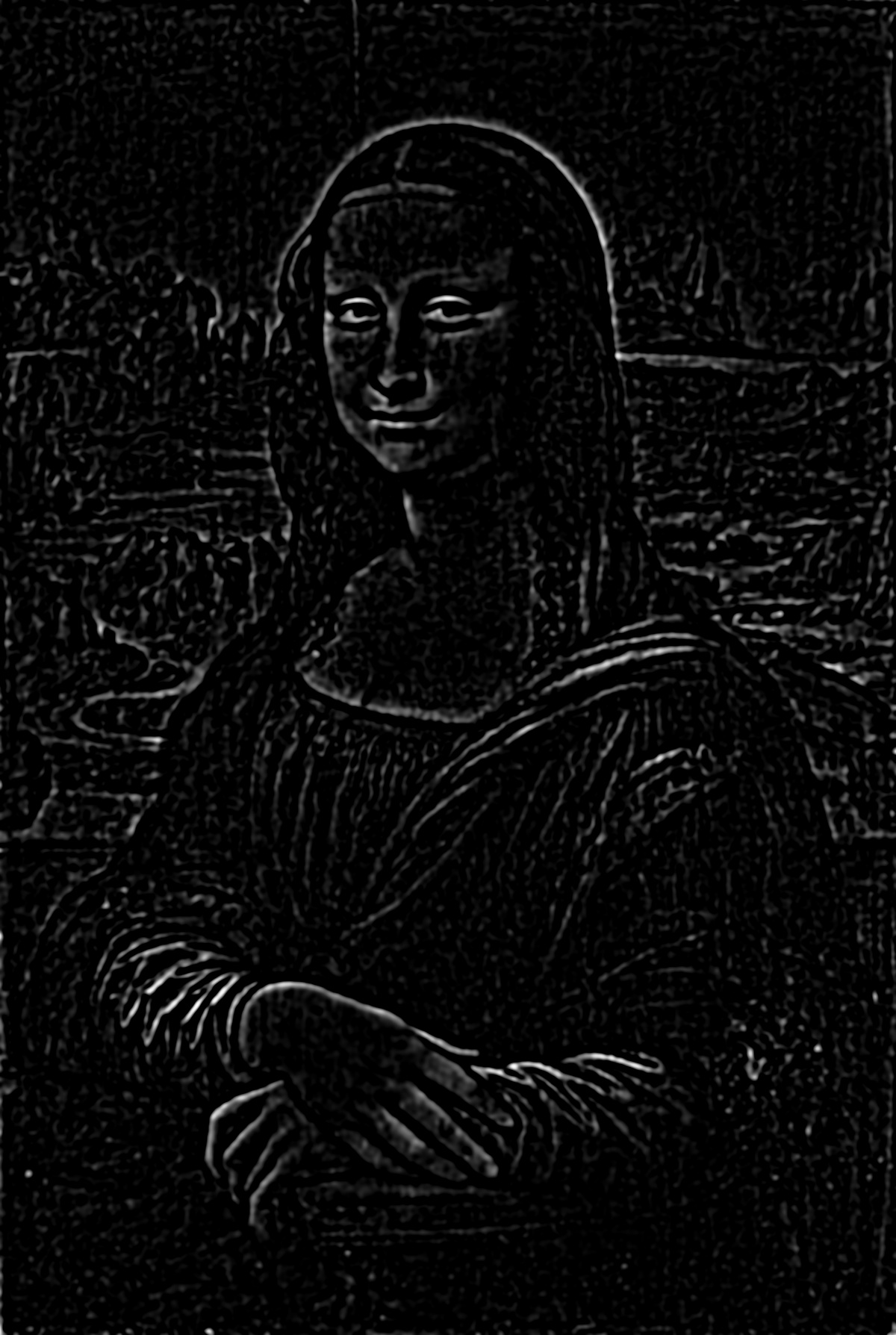
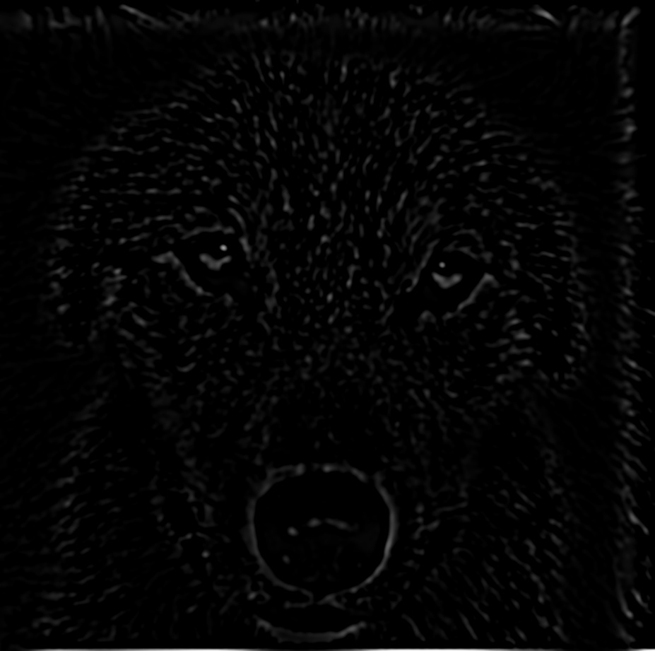
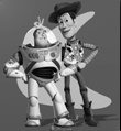
Original, highpass, sharpened
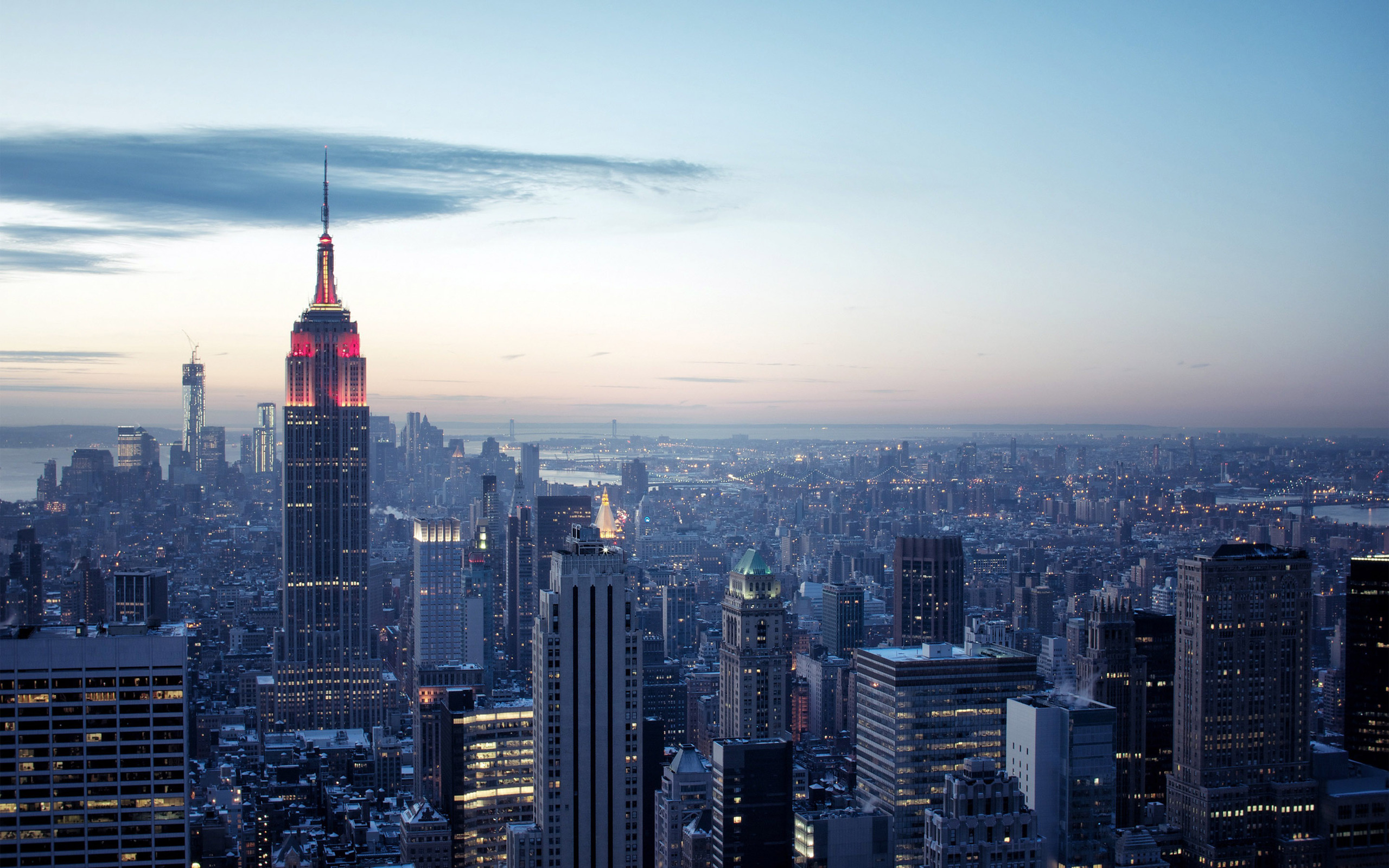
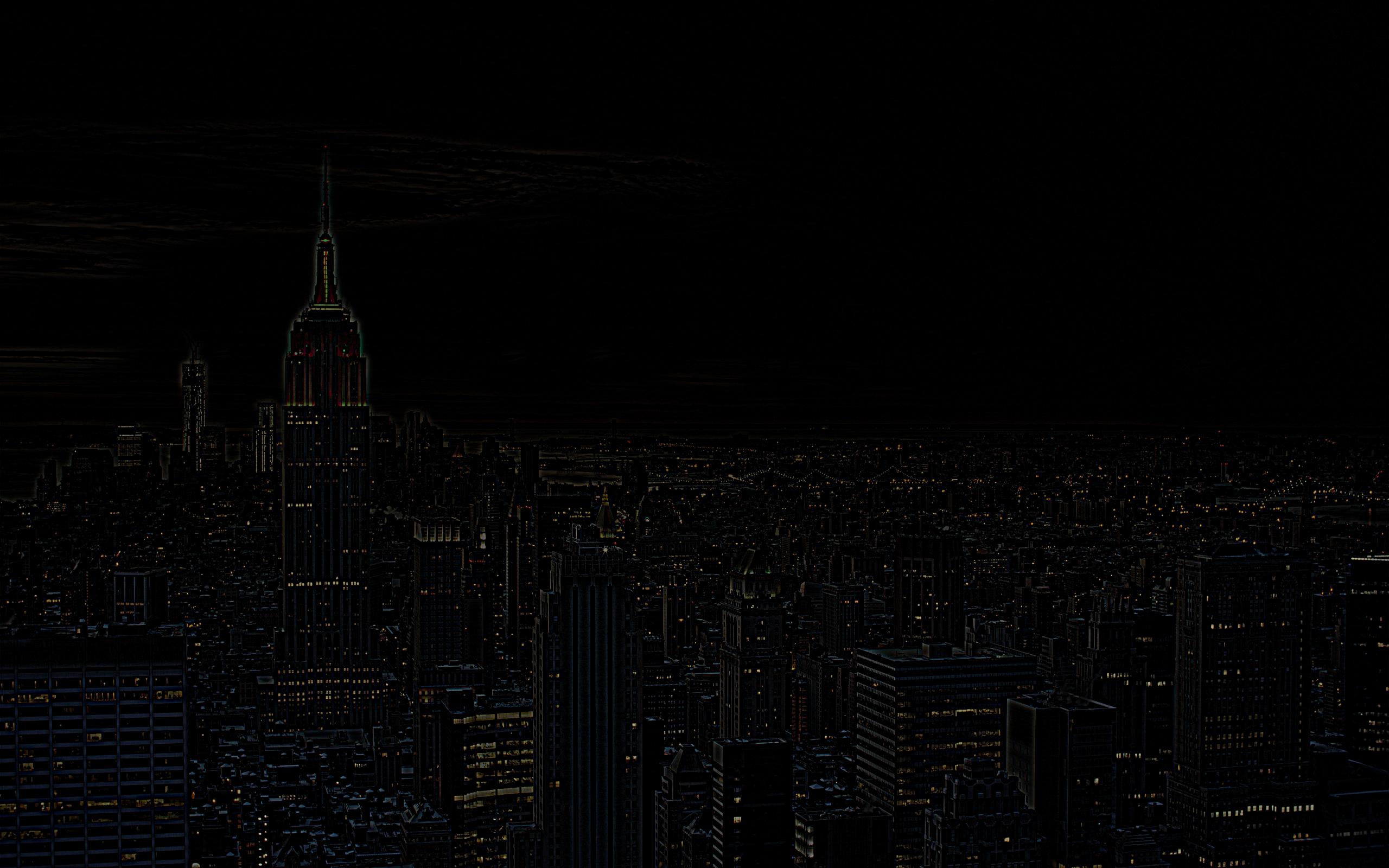
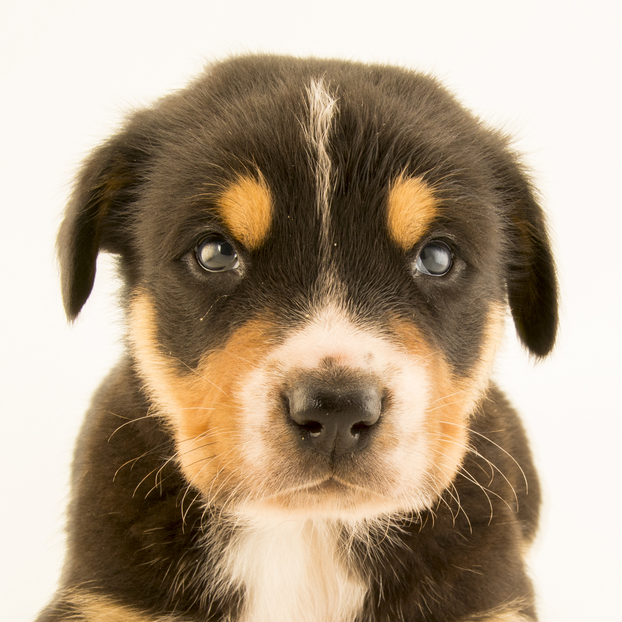
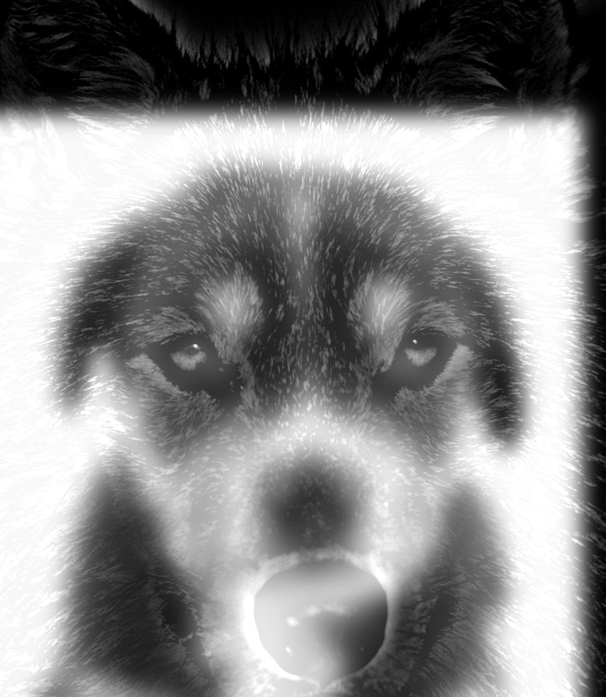
We used a technique called unsharp mask filter to sharpen our image. This is done by gaussian blurring the image to obtain the low-pass frequency image and then subtract the low-pass with the original image to obtain the high-pass frequency image. Lastly, the sum of the original and high frequency images multiplied by a scalar (let’s call it s) to get a sharpened image. The scalar s determines the level of sharpness the final image will have. sharpened = original + s*(original - blurred)
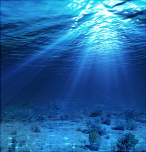
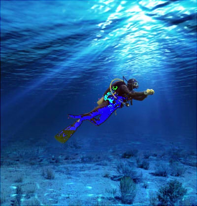
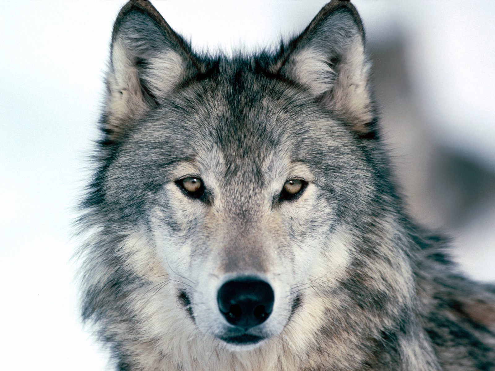
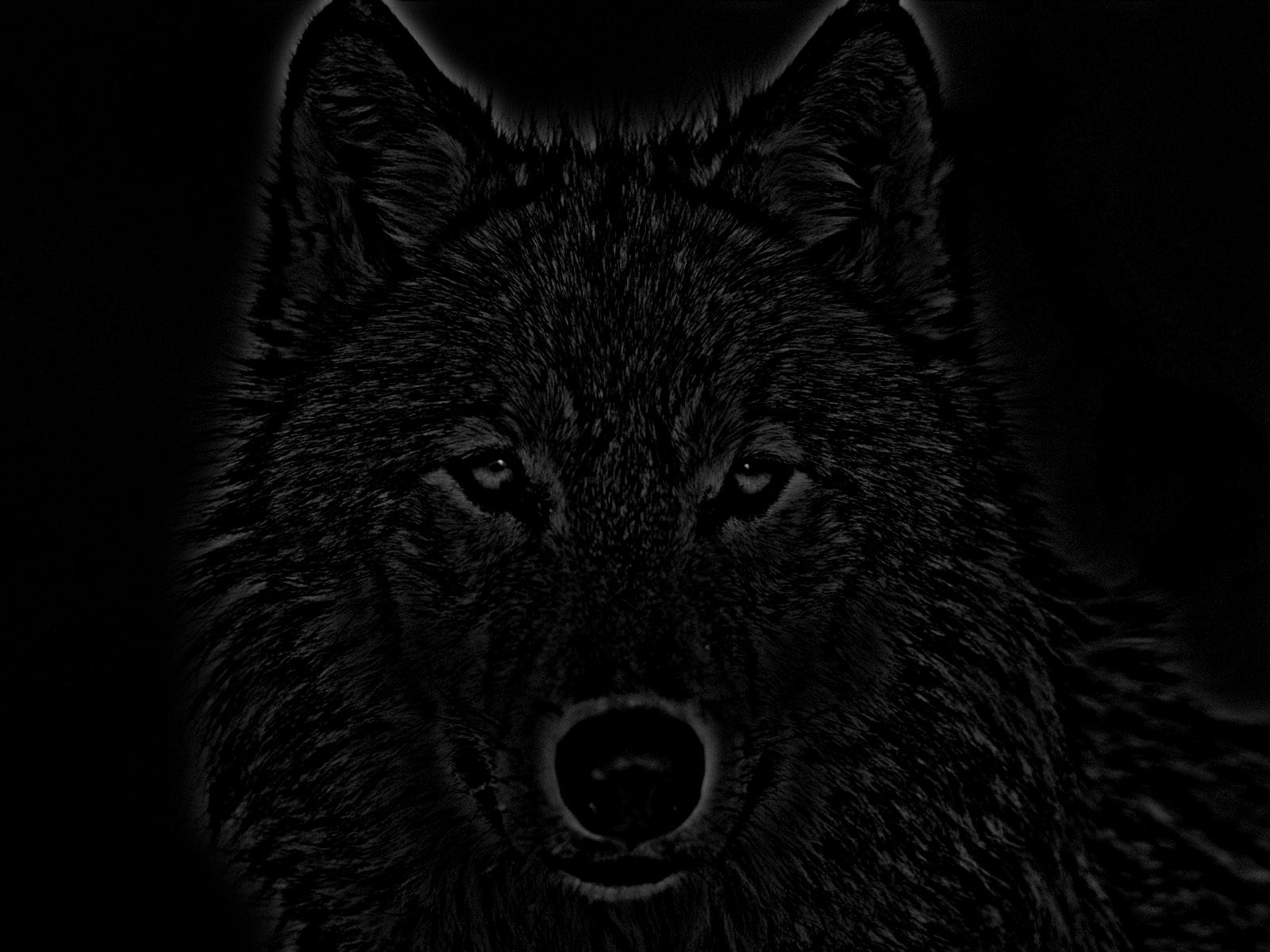
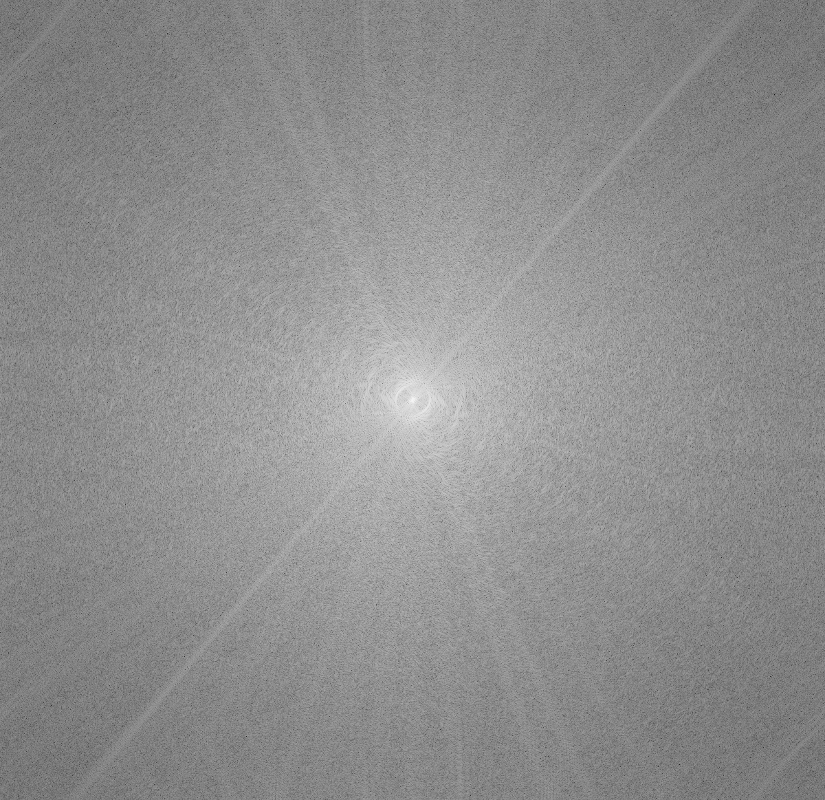
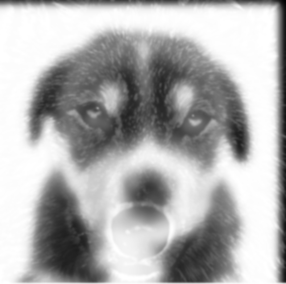
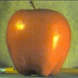
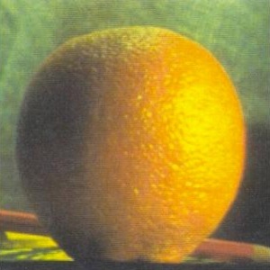
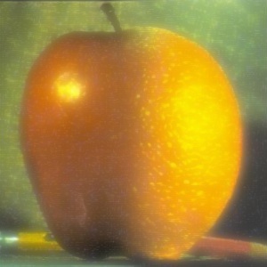
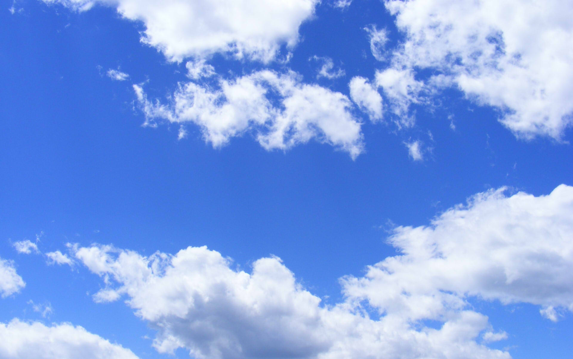
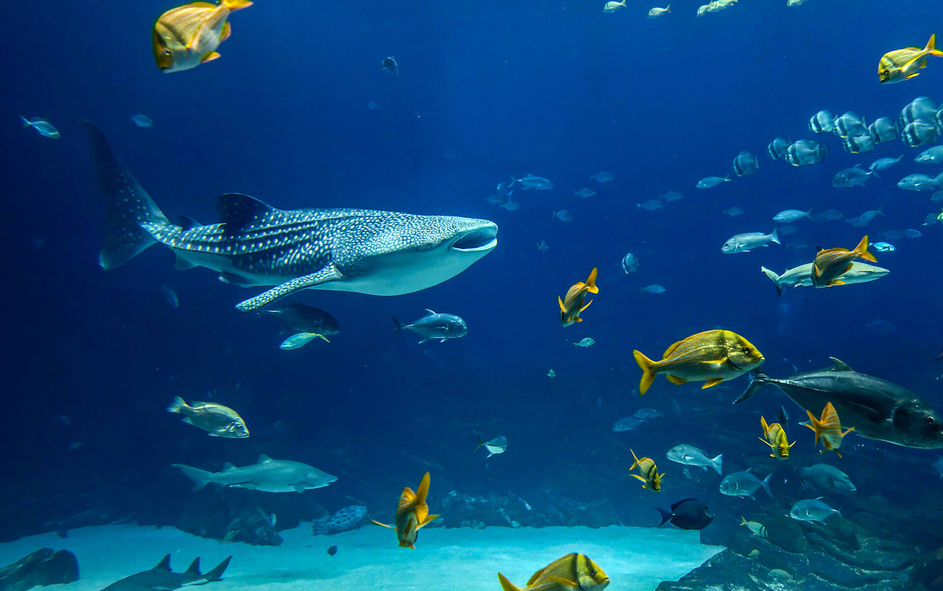
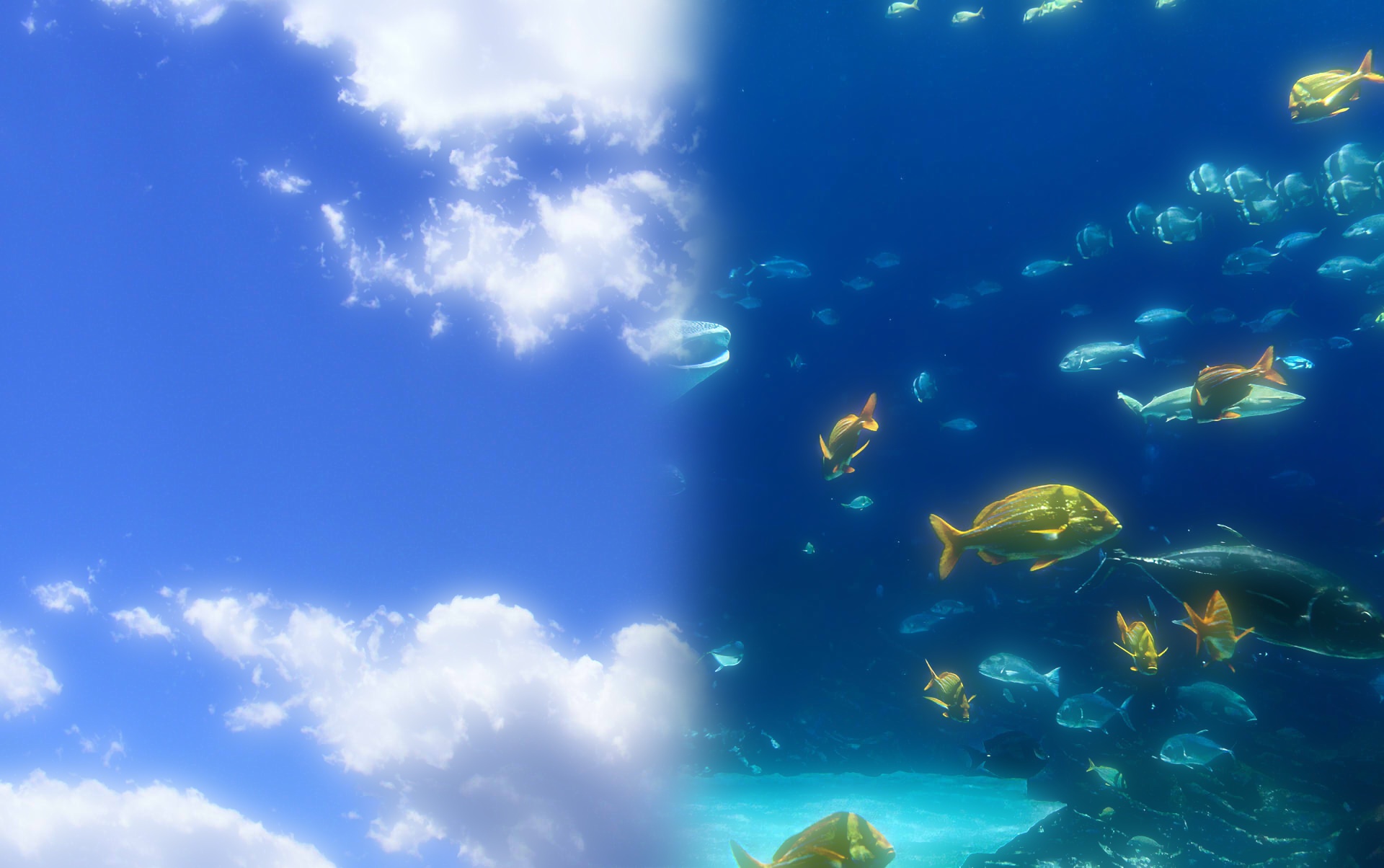
We generated hybrid images by blending a low-pass filtered image with a high-pass filtered image. To create these images, we take two photos and then filter out the low frequencies in one photo and the high frequencies in the other photo. We then align and layer the two filtered images and stack them on top of each other. The goal is to show that high frequency tends to dominate perception when up close. As the distance from the viewer to the image increases, the lower frequencies become more noticable.
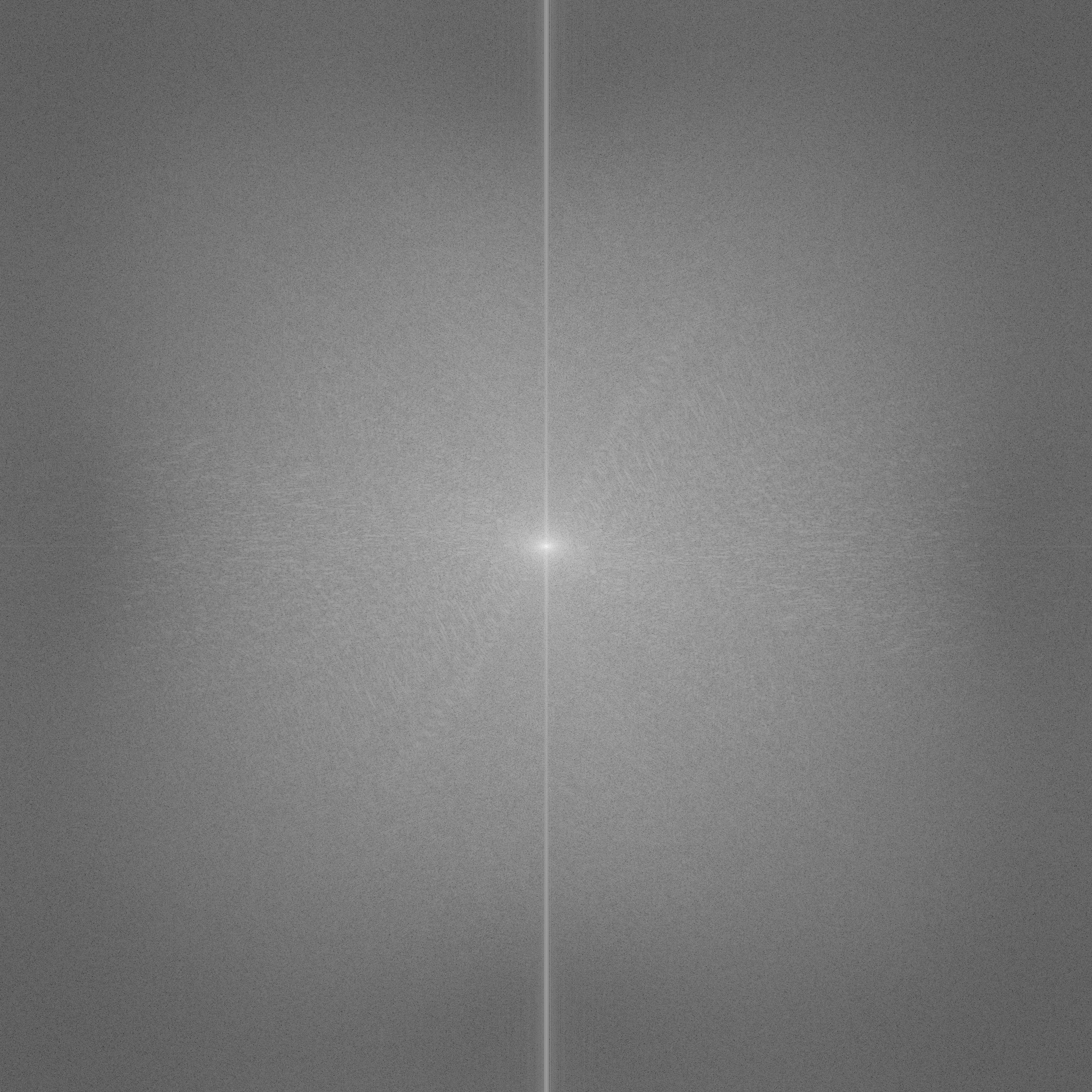
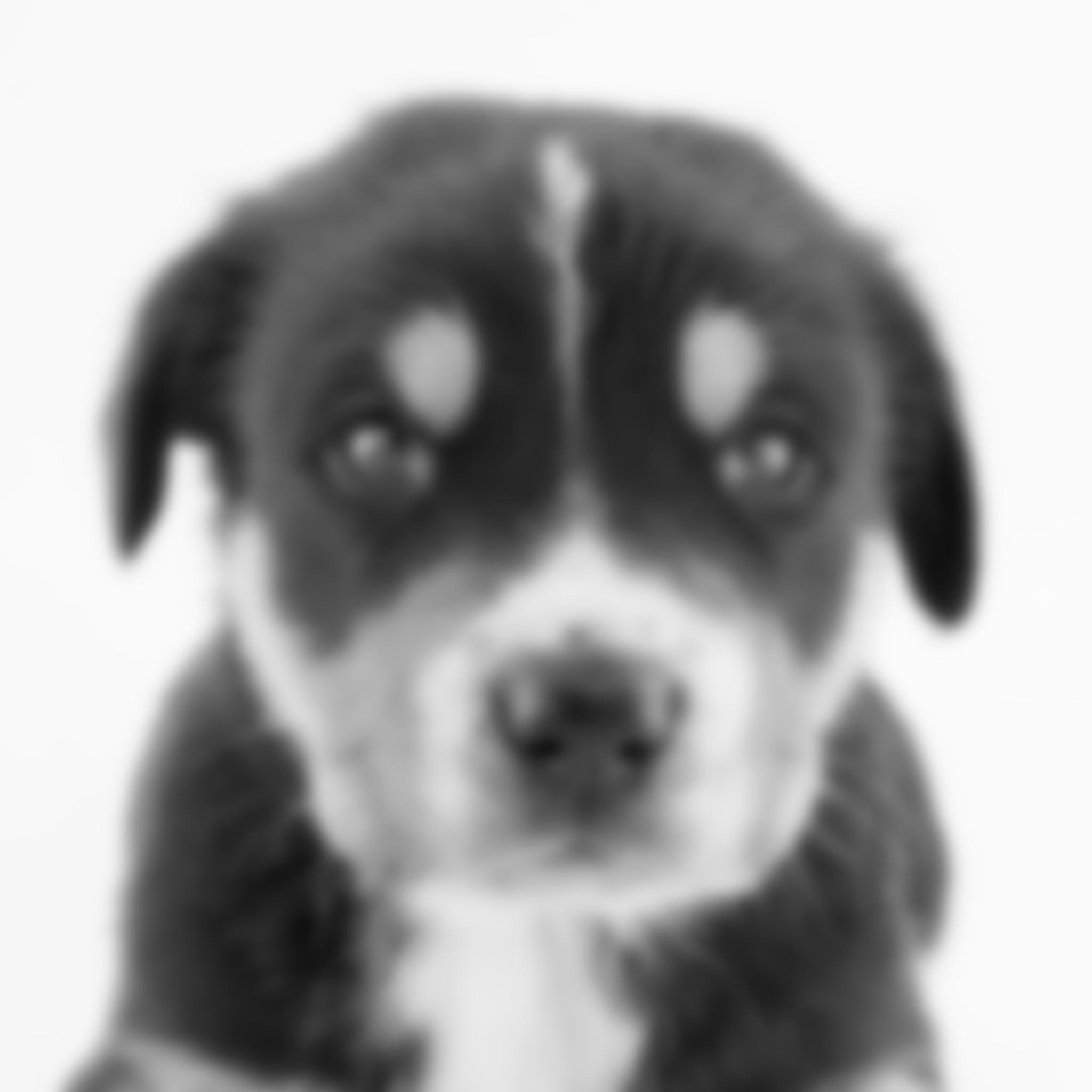

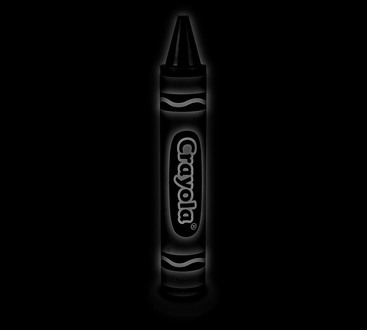


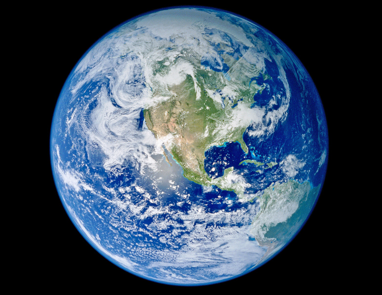


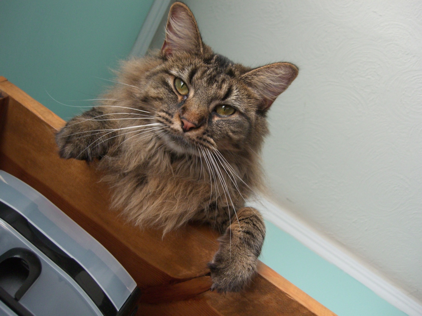
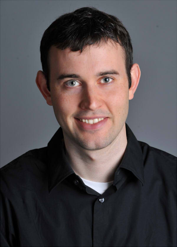
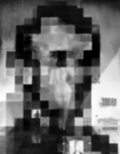
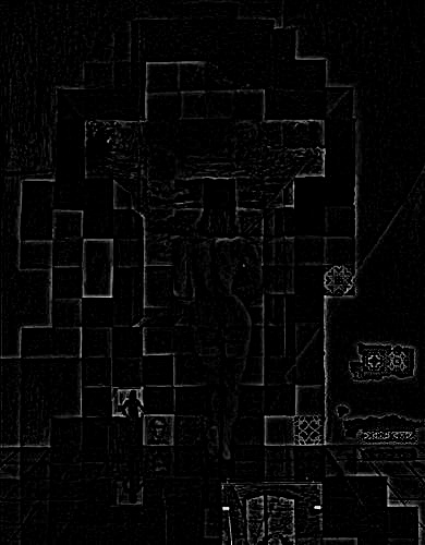
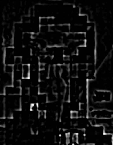
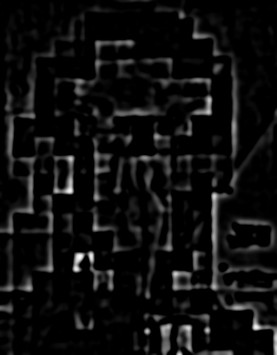
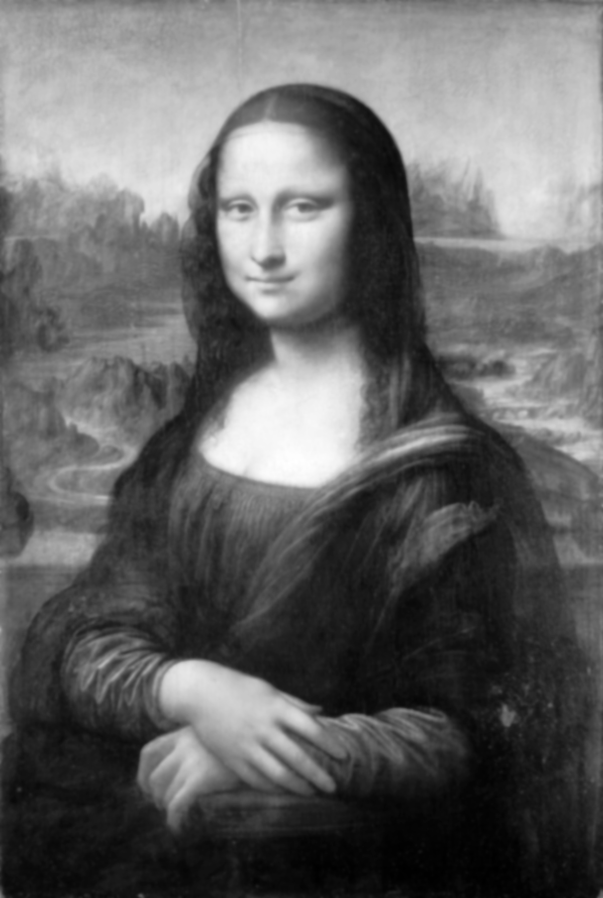
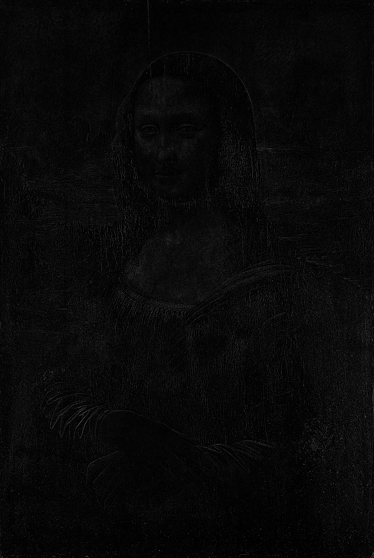
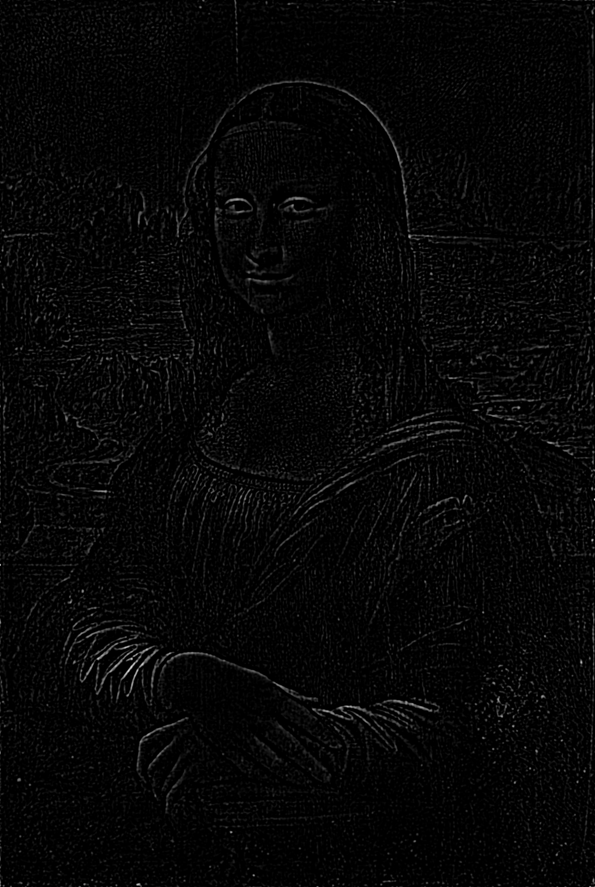
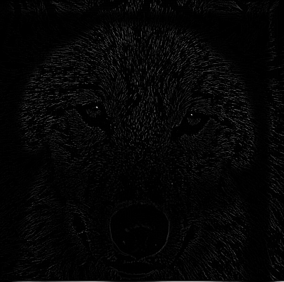
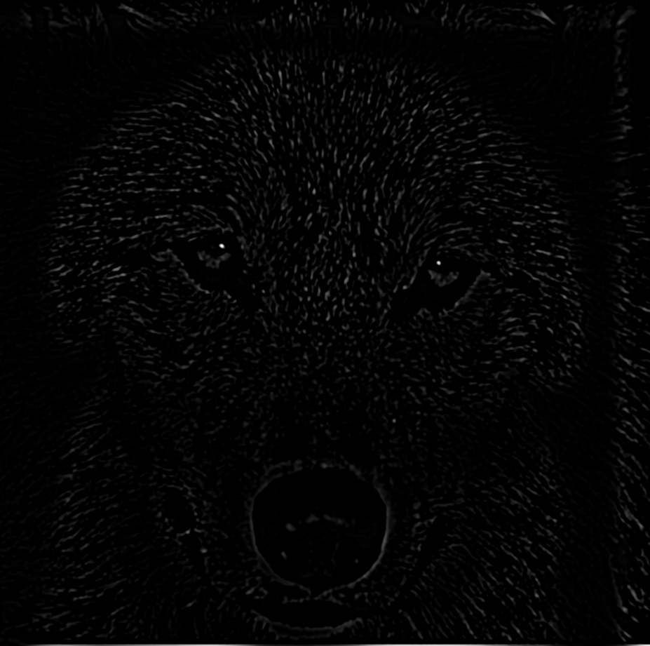
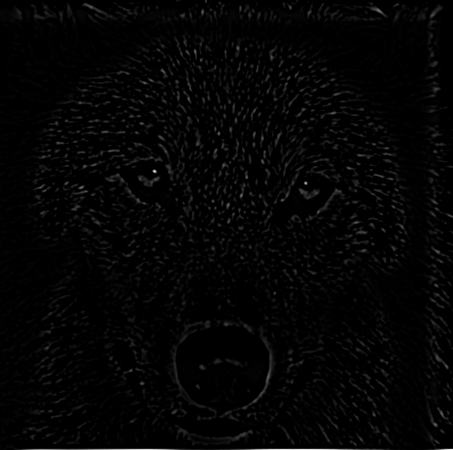
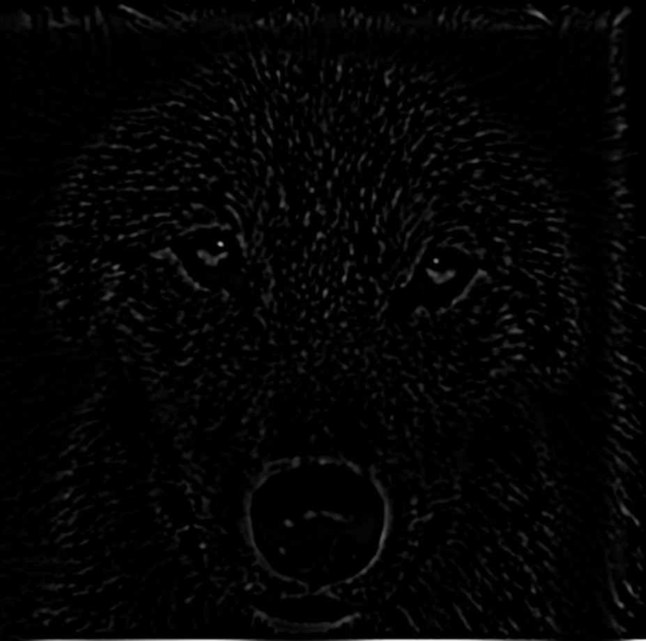
The pictures below are examples of the gaussian and laplacian stacks at different levels. Unlike pyramids, stacks does not downsample. Gaussian filters smooth the image and Laplacian images bring out the sharper edges. By combining gaussian and laplacian of two images, we were able to generate hybrid images in the last part


When merging two images without any further actions, at the place where the two images connect. a vivid seam can be seen between them. Through the technique called Multiresolution blending, we use of gaussian and laplacian stacks to generate a more smoother merge. With the laplacian stacks of the two images, at each level, we generate a new image through the formula LA * M + LB * (1-M). LA is the laplacian of image 1 and LB is the laplacian of image 2 at the current level. Once we gone through all the levels of the stack, we combine all the newly generate images to get a new out high frequency image of the merge. Finaly, we add back in a level of gaussian of a merge between the two images to obtain the final image with a gentle seam between the two images


The goal for this part was to reconstruct the sample image shown below by first computing its x and y gradients as well as one refernce pixel. We then setting up a system of linear equation with these data and solve it using least squares. The following results can then be used to reconstruct the original image.
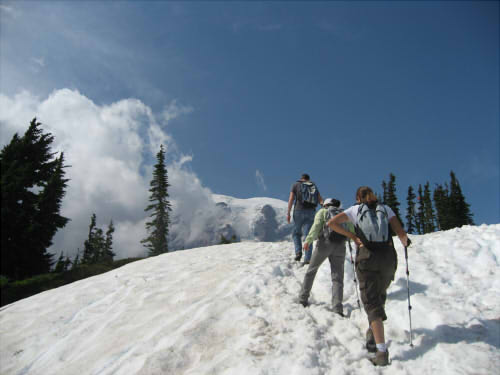
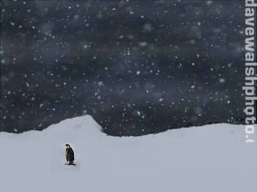
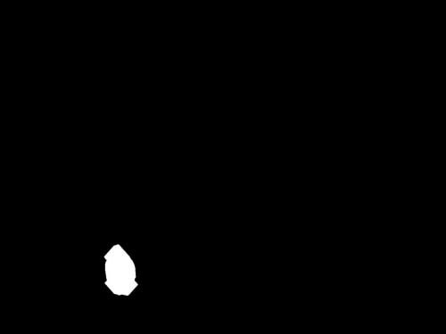
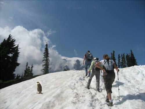
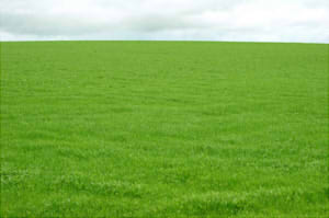
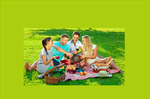
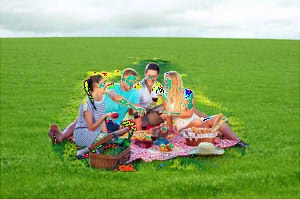
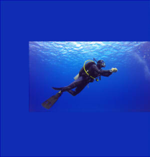
The goal for this part was to seamlessly blend a source image into some location within a target image while also adjusting to the target images using gradients. The method used in this part is similar to the to the method described in the toy problem above. We pick two images, a source and a target, create a mask of thet area we want to add to the target in the source image, and then within the mask blend together using the gradients of the images in a process called Poisson Blending.