Computational Photography: Face Morphing and Modelling a Photo Collection
Aneesh Akella
Introduction
The purpose of this project was to develop a technique for face morphing. Assuming two images, Image A and Image B, Delaunay triangulation was used to create a visual transformation from one image to another. Rather than simply cross dissolve, the triangulation would allow the visual transformation of the shapes in Image A to the shapes in Image B. Not only was it used to transform images, Delaunay triangulation was also used to change face geometry. Cross-dissolve techniques were utilized to allow for color-change. Further details will be provided below.
Half-Way Test
Before creating a full transformation from one image to another, a half-way image should be calculated to test whether the transformation is occurring in both the shapes and the colors.
Images
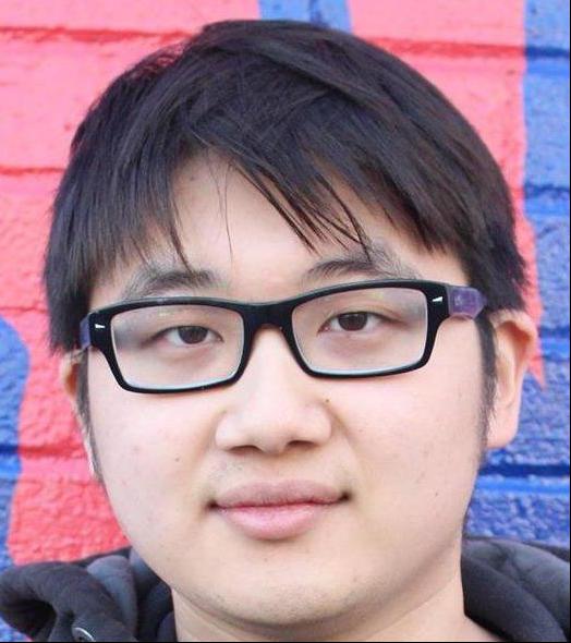
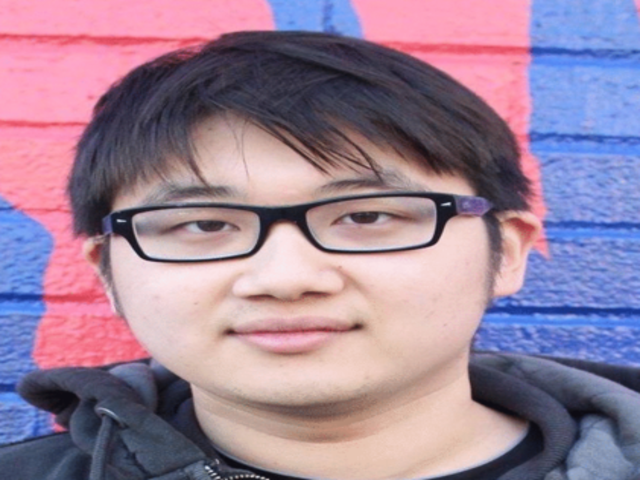
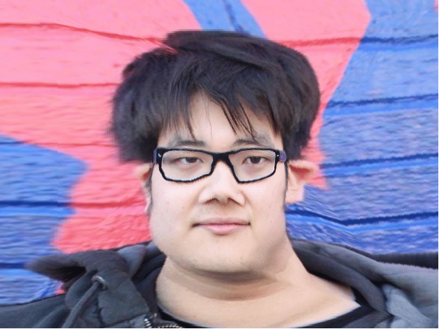
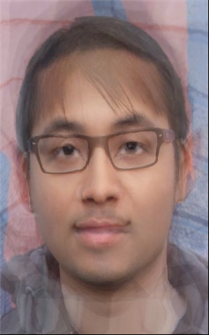
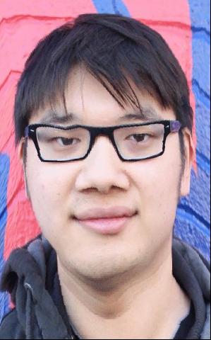
My roomate, Ki
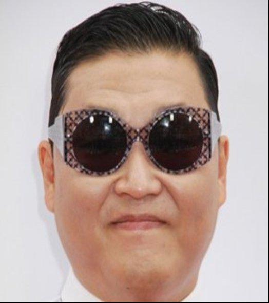
The signer, Psy
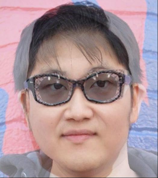
Their Halfway Image
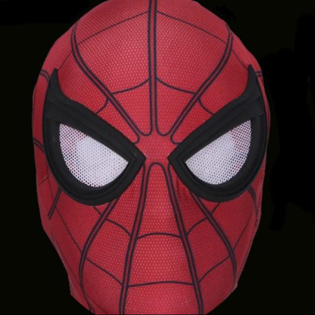
Spiderman
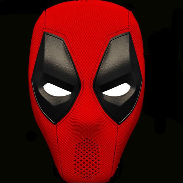
Deadpool
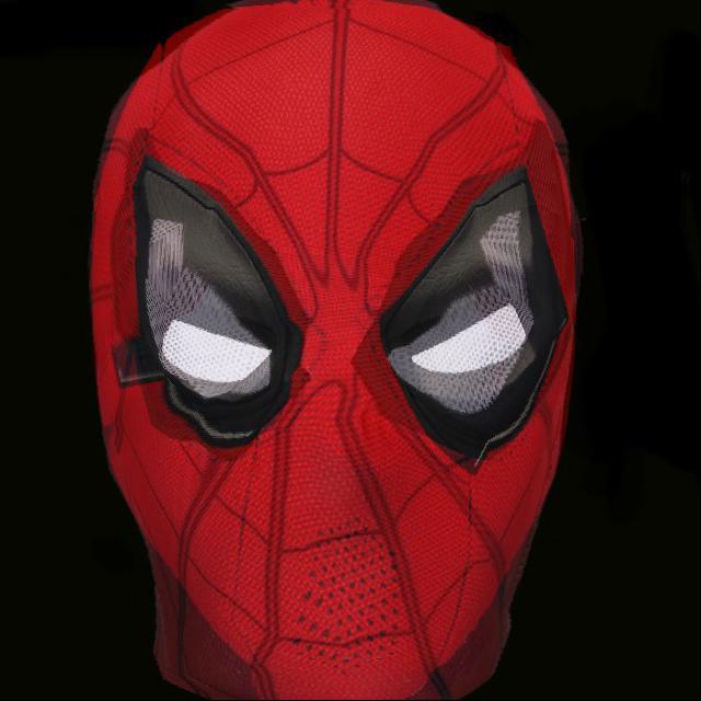
Their Halfway Image
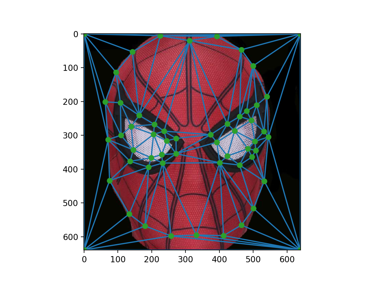
Spiderman Mapping
Half-Way Mapping
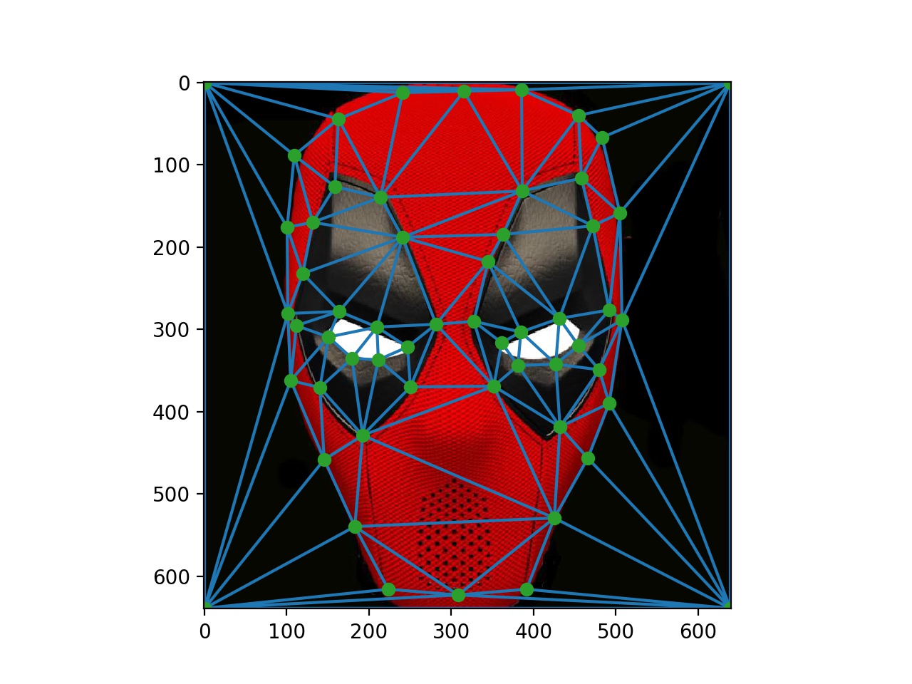
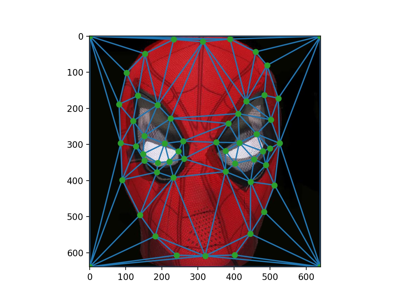
Deadpool Mapping
Image Morphing
Once the half-way image has been constructed, we can design a full image morph. First, features on the source image and transfer image are mapped by selecting points on the image. By selecting an equal number of corresponding points on each image, a Delaunay triangulation mesh can be constructed.
Since the point is to create an animated morphing sequence, the shape does not immediately change from Shape A to Shape B. Rather it is a slightly gradual transition. To display this transition, we need to average the triangulation meshes.
The equation looks like this: average_mesh = (1 – a) * soure_image_mesh + a * transfer_image_mesh, where a is the warp factor that ranges from 0 to 1. At the initial image, the warp factor is 0 and has its original shape. However, by the end of the sequence, the warp factor will be 1. At this point, the image should have the transfer image’s shape. To create this steady transition, a series of images with the warp factor varied from 0 to 1 are gathered. For the gif below, the warp factor was varied by 2 for each image.
Once we calculate the average mesh, we should add pixels from the source and transfer images to the average. To figure out which pixels go where, we create two affine transformation matrices at each triangle—one that maps the pixels in the average image to the source and the other mapping the pixels in the average image to the transfer image. If a pixel falls into a given triangle, the inverse affine transformations of the pixels in the average image are taken to find the source and transfer pixels.
Through this process we are able to create, the morphing sequences down below. Cross dissolving was done in a similar way: average_color = (1 – t) * soure_image + t * transfer_image, where t represents the color factor.
Image Morphing
Spiderman to Deadpool

Ki to Psy
Mean Face
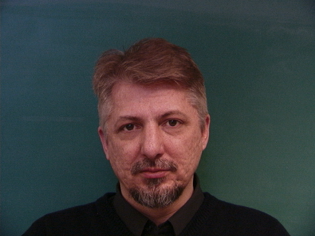
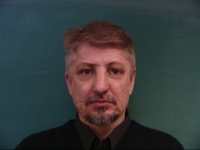
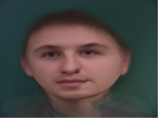
Given a dataset of Danish scientists with feature points already mapped, we can compute the average face of the Danish computer scientist. First, the average shape should be computed. For the 37 images, a triangular mesh for each image was constructed. These were averaged to produce an average mesh. Then, for each image, we transformed the face geometry of each image with the average mesh. However, the cross dissolve factor was left at 0, while the warp factor was changed to 1. This will change the shape of the face, but will prevent the magnitude of the pixel colors from changing. Herego, we create a face warp. After a face warp has been made for all 37 images, we add up all the warped images and average them to create the average Danish computer scientist image below.
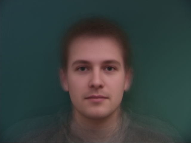
Average Face from Dataset
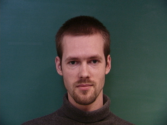
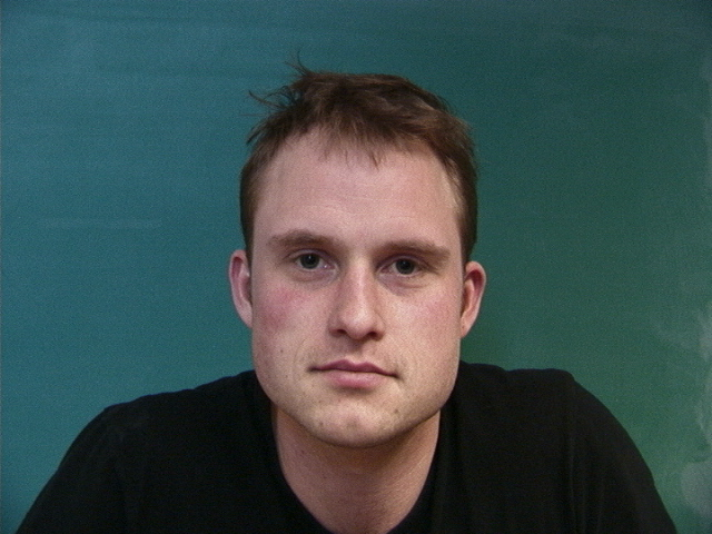
Sample Faces from Dataset
Transformed Faces
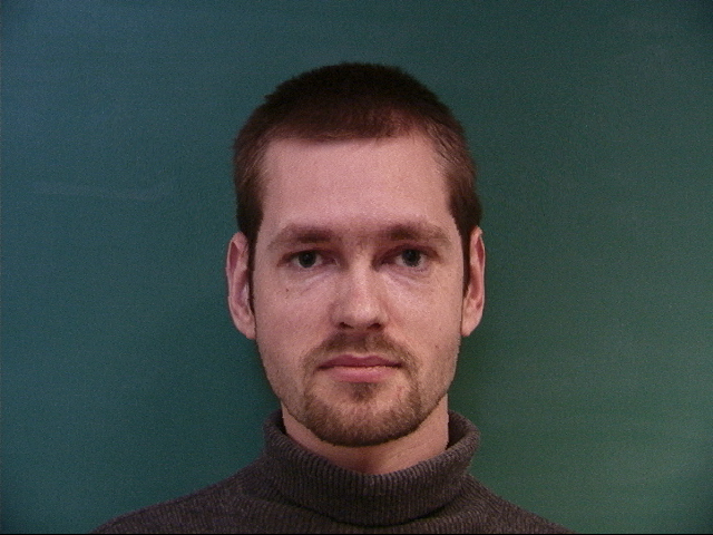
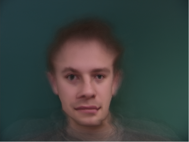
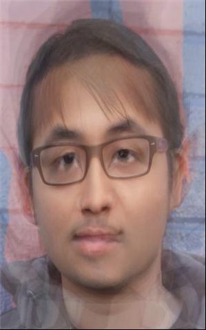
My face transformed to Danish Geometry and vice versa
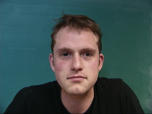
Ki's face transformed to Danish Geometry and vice versa
Now that, we have a picture of the average Danish computer scientist, it is now possible to morph my face’s geometry into that of the Danish computer scientist. If you look at my morphed image, you can see my nose got more narrow and my cheeks are more fuller, similar to the Danish guy. If you look at the Danish computer scientist, his facial structure become more like mine: his nose expanded, his head got more narrow, and a semblance of smile formed on his face.
If you look at Ki’s morphed face, you can see it got significantly skinnier. His smile is also more similar to the Danish computer scientist’s smile. The Danish guy’s face, on the other hand, ballooned up. His facial structures are also more in line with Ki’s facial structures.
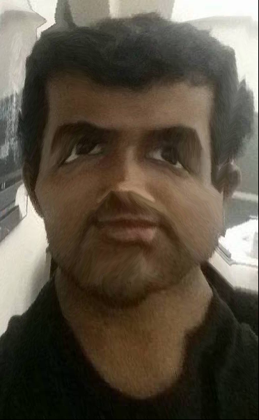
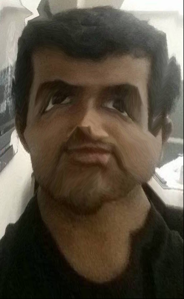
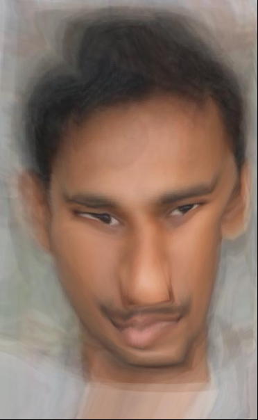
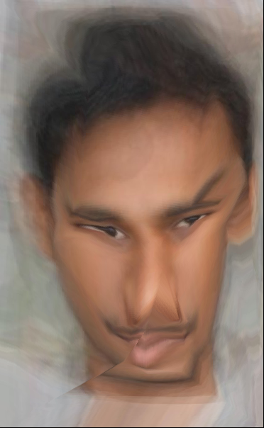
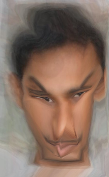
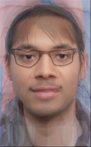
Caricatures
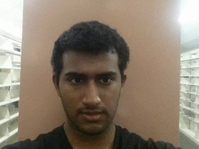
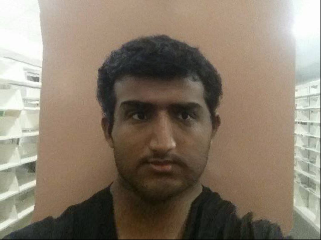
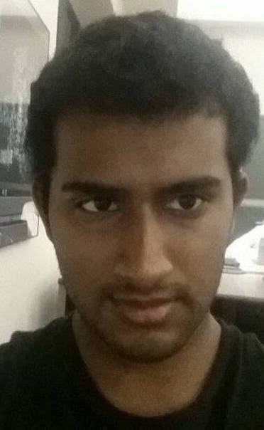
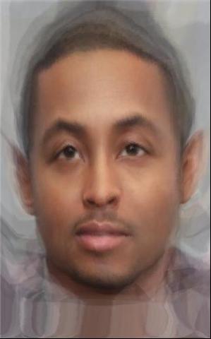
If we set the warp factor to above 1, and set the cross-dissolve to 0, we can create caricatures. In other words, we can get a reduction of the original facial features and instead get an intensification of the features in the transfer image. In my example, the transfer image is an average south Indian guy. If you look at the photos above, as the warp factor increases, my mouth raises higher and my nose becomes skinnier. I almost gain more of a poker face look – similar to the picture of the Indian guy.
The Indian guy, on the other hand, now has a much larger nose, his facial shape is more similar, and he now is slightly smiling. As we intensify the warp factor, his smile accentuates, the nose becomes even bigger, and the face becomes a tad skinnier.
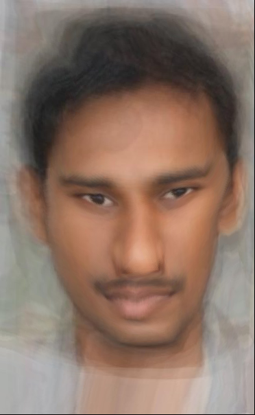
Original Images
Me
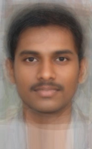
Average South Indian Male
Transformed Images
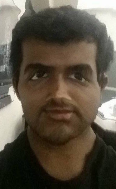
α = 1
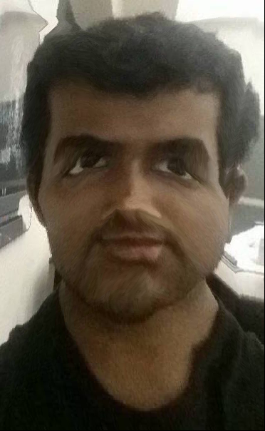
α = 1.25
α = 1.5
α = 1.75
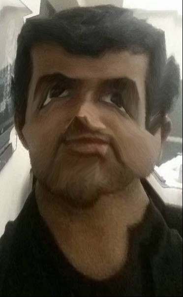
α = 2
α = 1
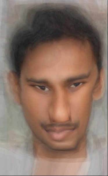
α = 1.25
α = 1.5
α = 1.75
α = 2
Bells and Whistles: Race Change
I turned my roommate black. I set the warp factor to around 0.35 to maintain some of Ki’s facial structures and set the color factor to around 0.7 so we can give Ki a black guy’s skin tone. I am quite proud of the result.
Korean Ki
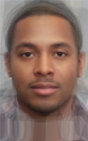
Average Black Male
Black Ki
Geometric Change: Warp Factor->0.35 Color -> 0
Color Change: Warp Factor->0 Color -> 0.7
Color Change: Warp Factor->0.35 Color -> 1
Color Change: Warp Factor->1 Color -> 0.7
Bells and Whistles: Friends/Multiple Video
Here is the link to my gif with Audio:
Bells and Whistles: Beier Neely Calculations
I decided to test the Beier Neely algorithm. The algorithm can be looked at here.
The main differences between Beier Neely and the mesh algorithm is that lines are used as inputs instead of points. Furthermore, the algorithm is more paramaterizable. There are three additional parameters: a, b, and p. The variable, a, determines how strong pixels close to the line will be. If a is low, and a pixel is close to or on the line, the pixel on the source/transfer will the be transfered on the corresponding line on the average image. b determines how different lines can affect a single pixel. Low values [0 - 0.5] mean that pixels will not be affected by multiple lines despite difference. High values means pixels will be affected by lines closer to the pixel. p determines how the length of the lines affects where the pixels are transfered. The larger p is, the larger importance longer lines will have in determining where pixels are transfered.
For a similar-size image, Biere Neely has a much higher complexity. The mesh algorithm probably runs in O(mn) where m and n are the dimmensions of the image. However, Biere Neely operates at O(mnt) where t is the number of lines. Thus, it takes much longer to generate an image. I had to reduce the quality of the image 4-fold in order to create a gif in a reasonable amount of time. However, because Beier Neely has more inputs, there are more ways, the output sequence can be controlled. The following image was produced with a = 0.5, b = 1, and p = 0. Lines were drawn around the eyes and around the mask.
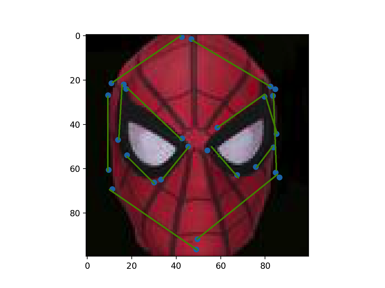
Spiderman Lines
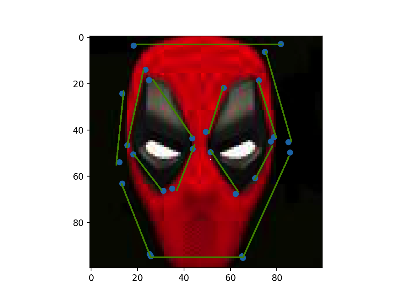
Deadpool Lines
Delaunay Mesh Morphing

Beier Neelay Morphing a = 0.5, b = 2 p = 0

Beier Neelay Morphing a = 0.5, b = 0.5 p = 0
Beier Neelay Morphing a = 0.5, b = 2 p = 1
The reason for the difference between the morphs has to do with the p values. When p is greater, larger lines have more importance. That is why the transition is smoother around the head for p = 1. You can see a low value of b results in a weaker transition.