PART 1

Overview

In this project, I took many overlapping photos, and stitched them together to form one image that contains all the information of all of the other images. In the following sections, I will describe the process which I took to create the Mosaic.

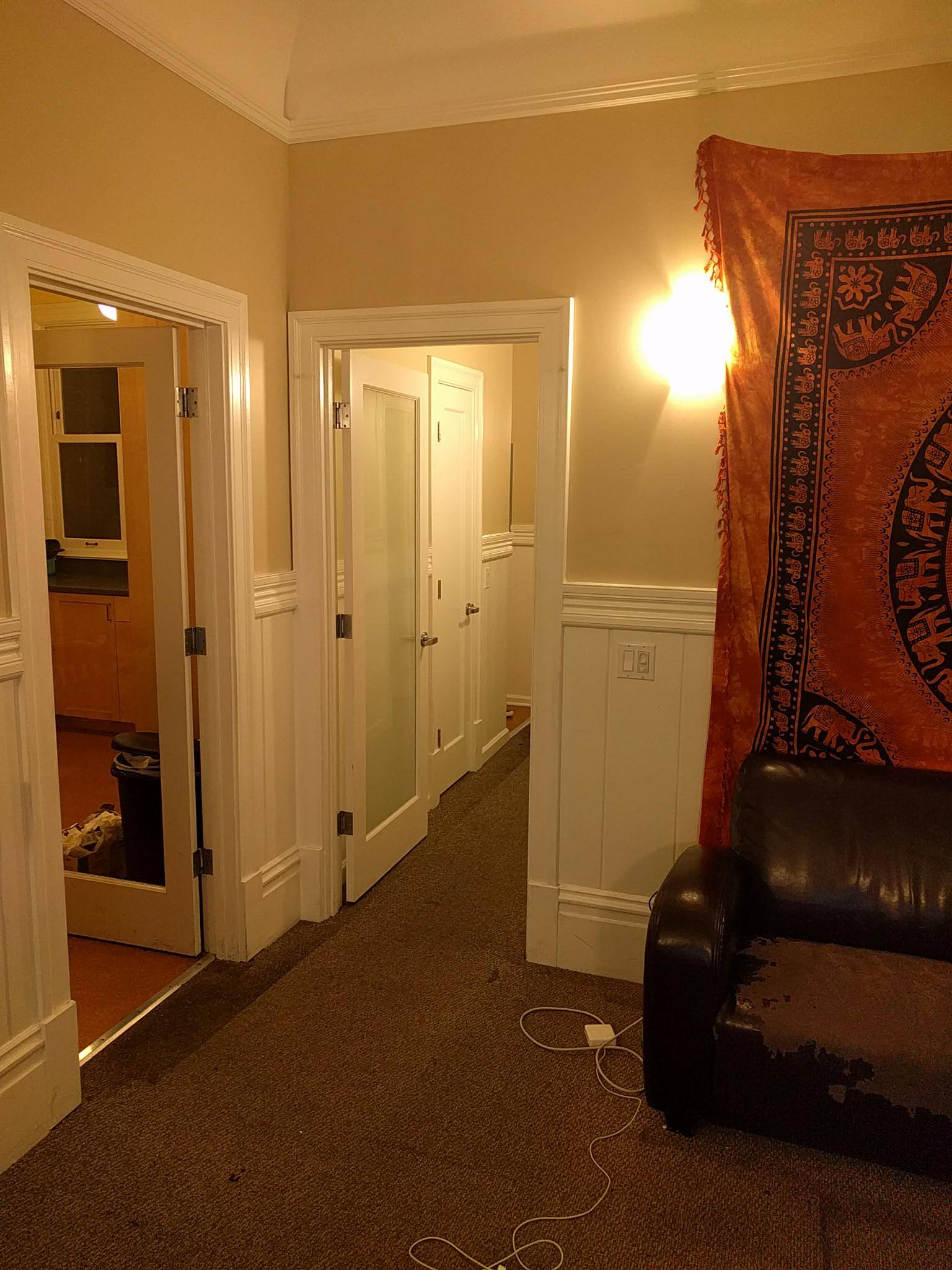
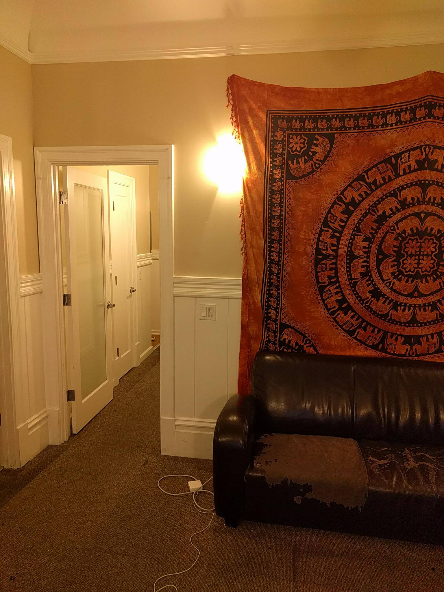
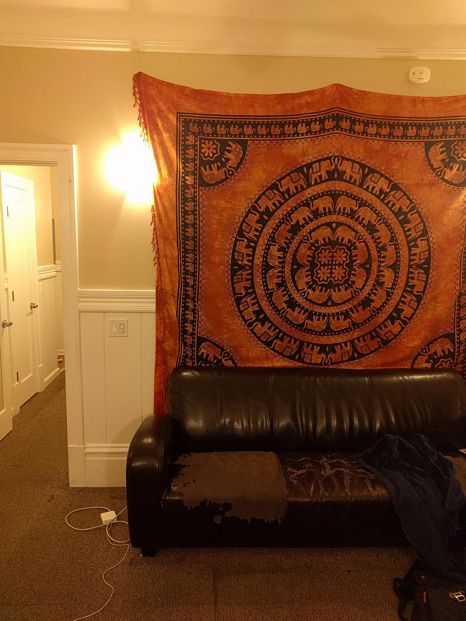
Shooting Pictures

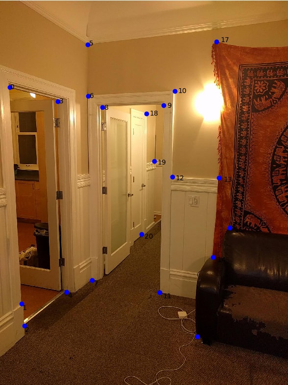
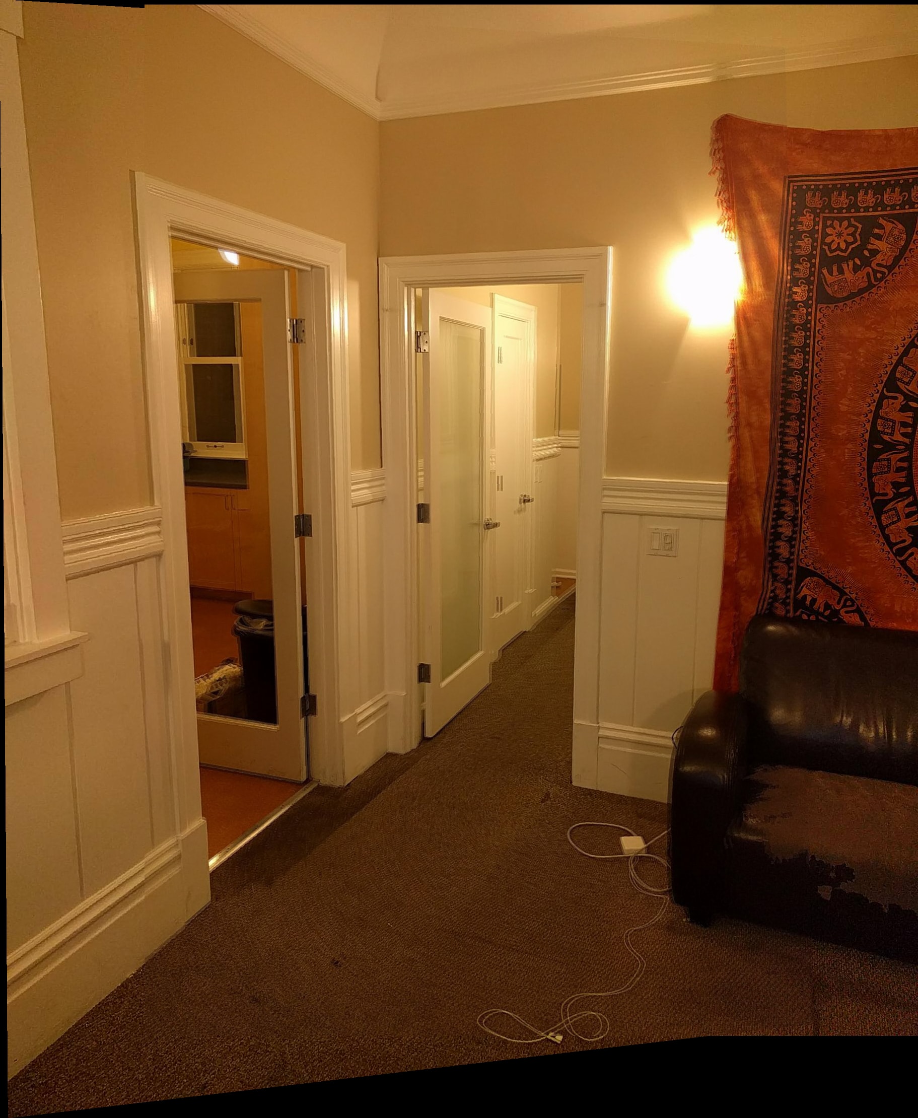
I took multiple pictures of the same scene, each shifted such that they overlap so I can find corresponding points to match.

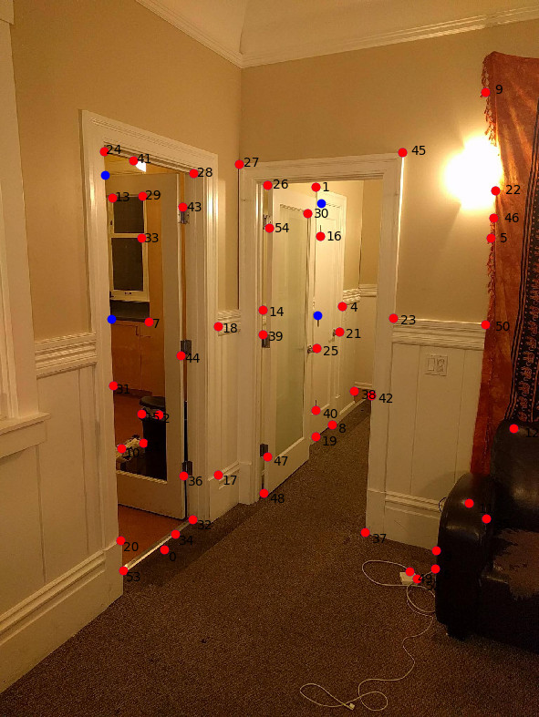
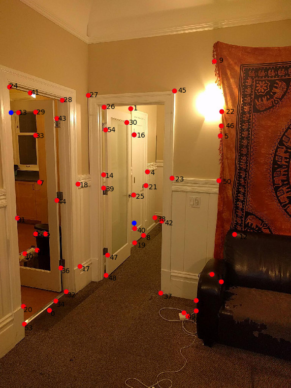
Selecting Points

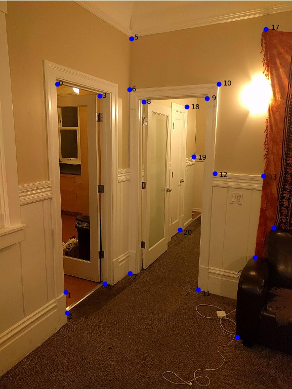
Recovering Homography

I defined a matrix H that transforms the point p to p'. Unlike the face morphing, the 3rd coordinate in p' is not exactly 1, since its warped onto a plane that is not parallel to z=1.

[a b c][px]   [wp'x]
[d e f][py] = [wp'y]
[g h 1][ 1]   [ w  ]
  

We solve for w:

w = g*px + h*py + 1
  

We substitute this back into wp'_x and wp'_y:

a*px + b*py + c = g*px*p'x + h*py*p'x + p'x
d*px + e*py + f = g*px*p'y + h*py*p'y + p'y
  

Finally, we can set up two equations like this for every pair of points and form a least squares problem, adding two rows for every pair of corresponding points.

                    [h1]
                    [h2]
                    [h3]
[xi yi 1 0 0 0 -xix'i -yix'i][h4] = [x'i]
[0 0 0 xi yi 1 -xiy'i -yiy'i][h5]   [y'i]
                    [h5]
                    [h6]
                    [h7]
                    [h8]
  

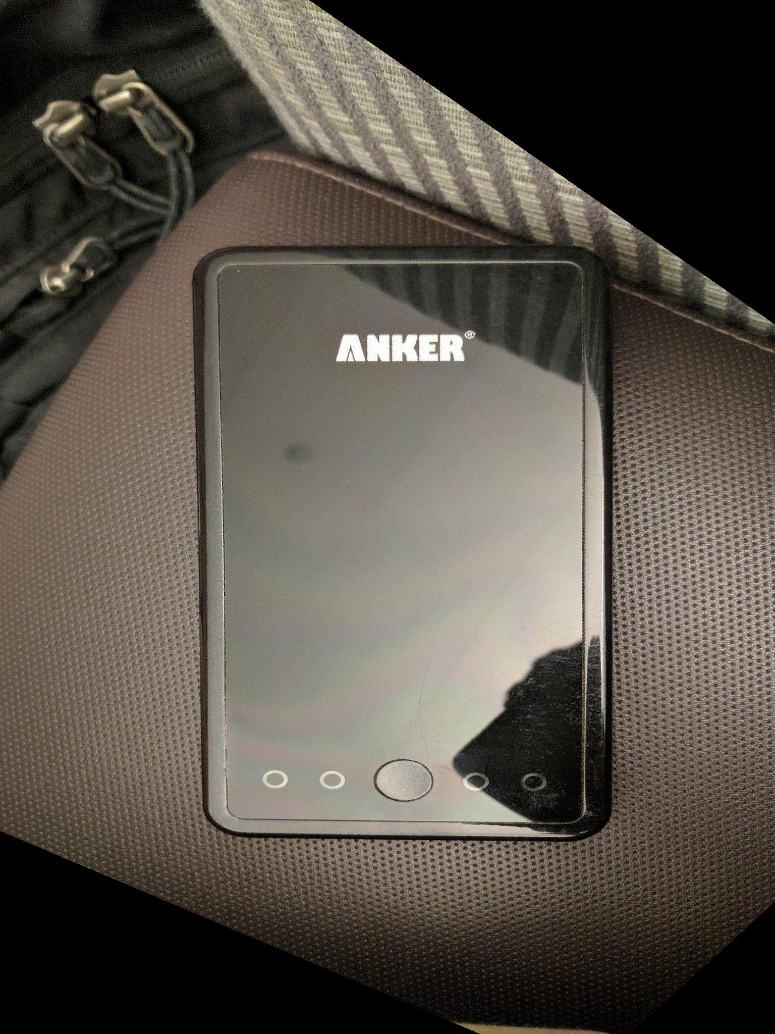
Image Rectification

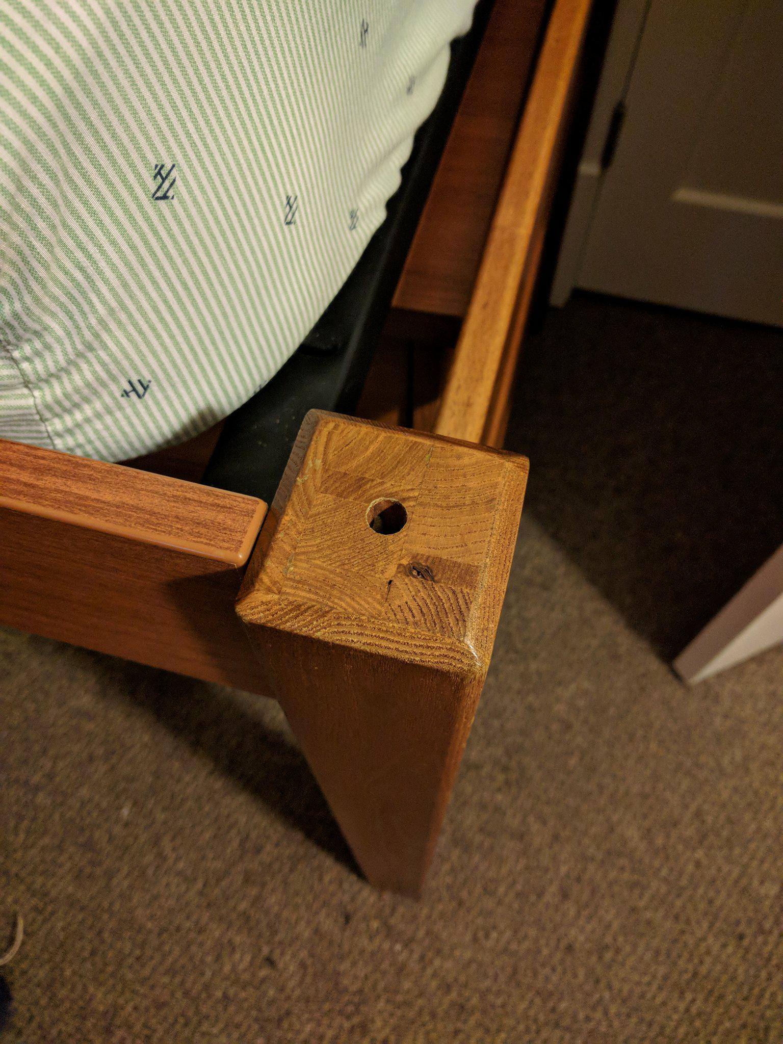
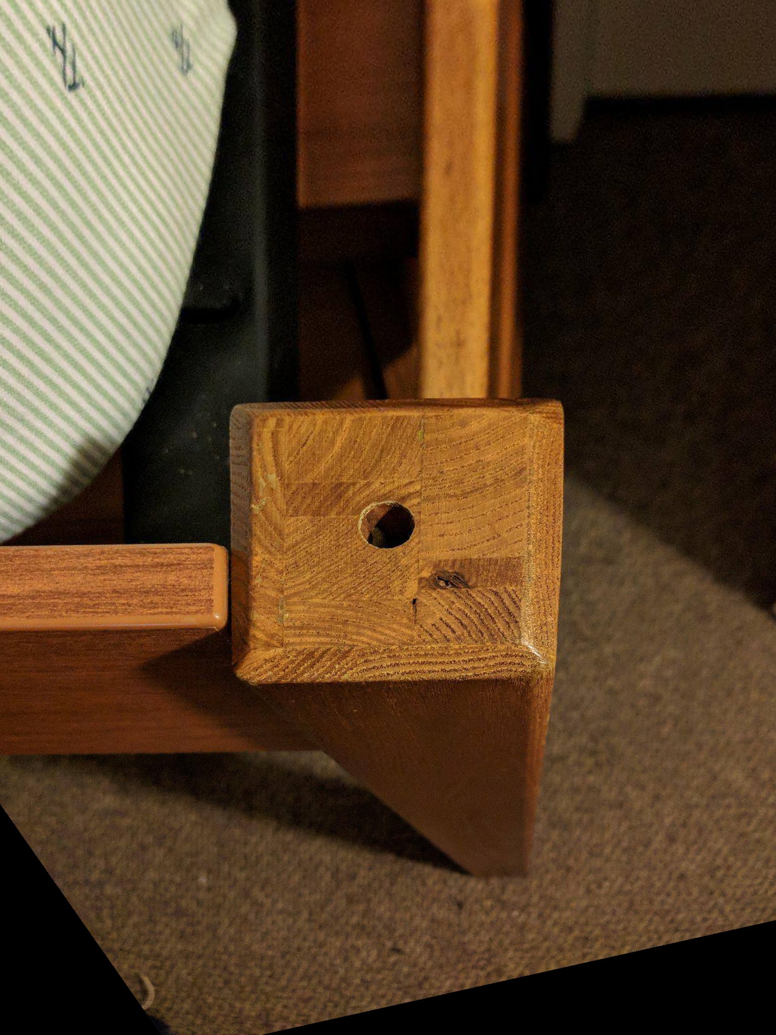
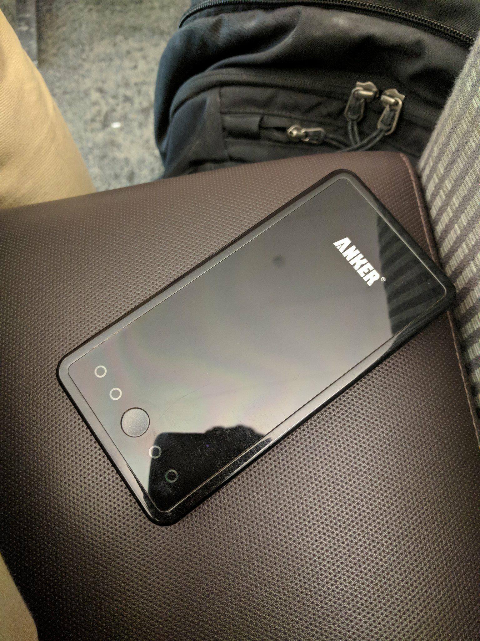
I took a picture of my bedpost, and a picture of my portable battery and warped them so that the post and battery was facing directly up and at 90 degree angles:

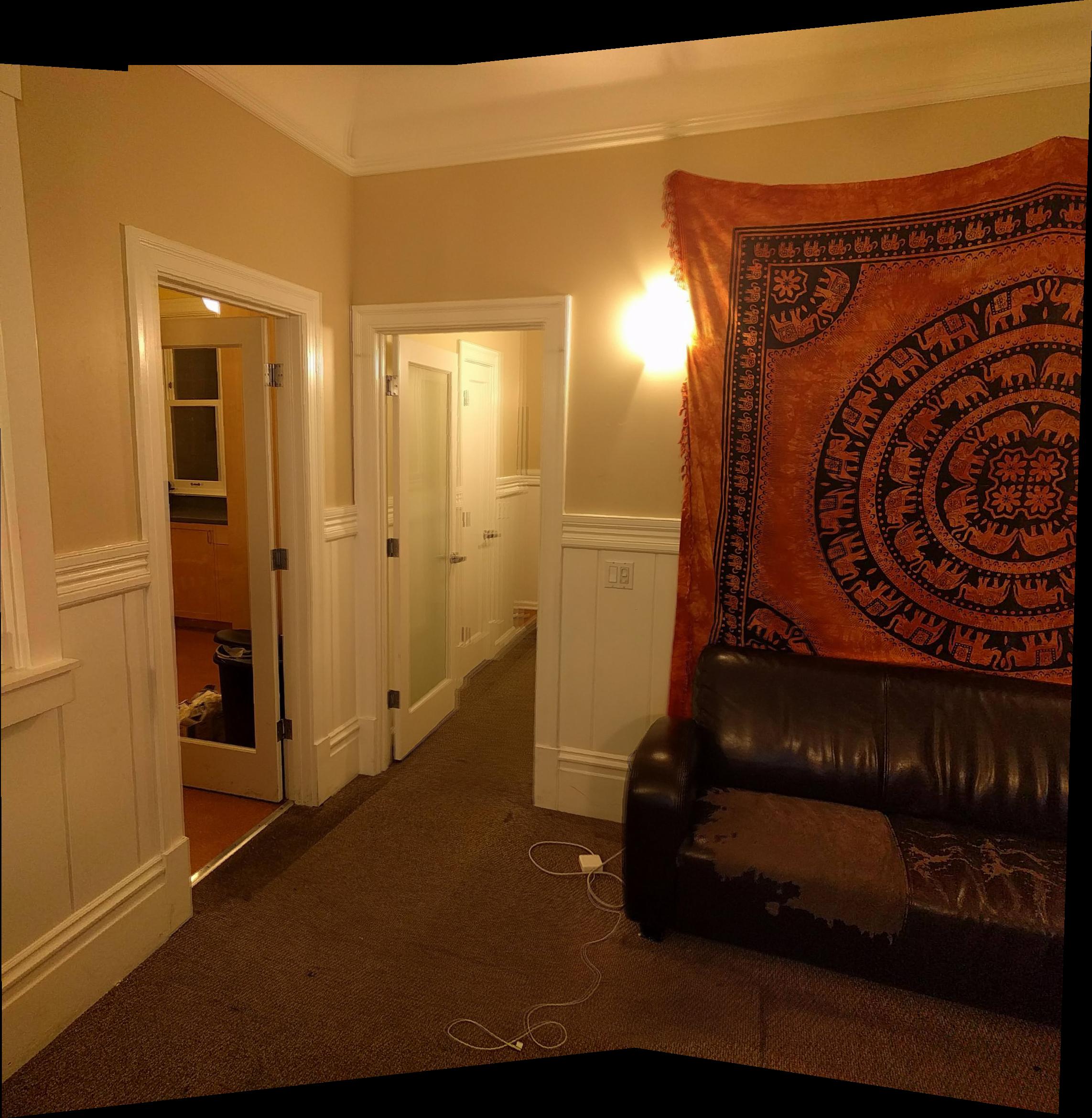
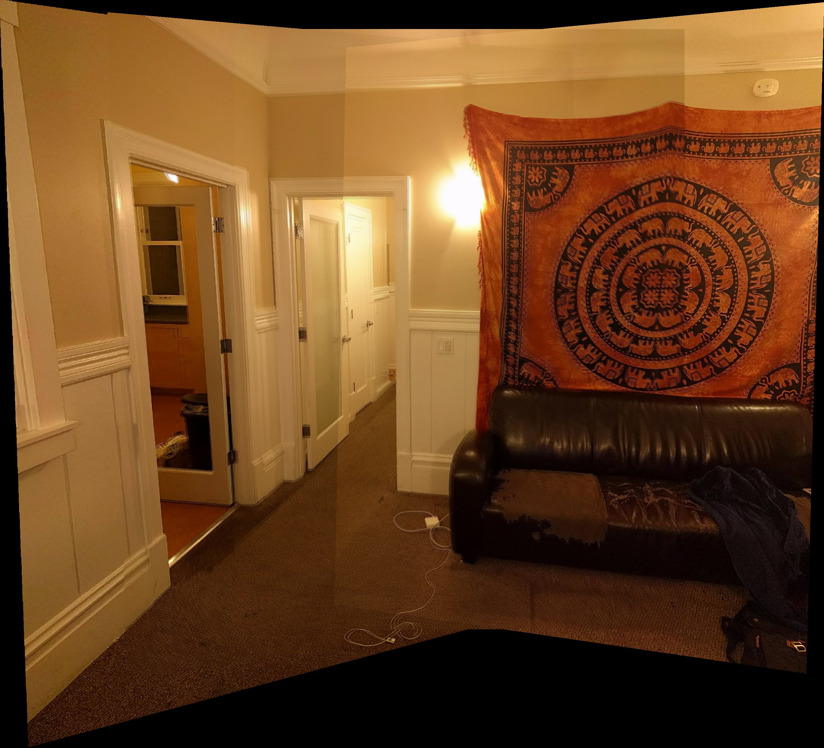
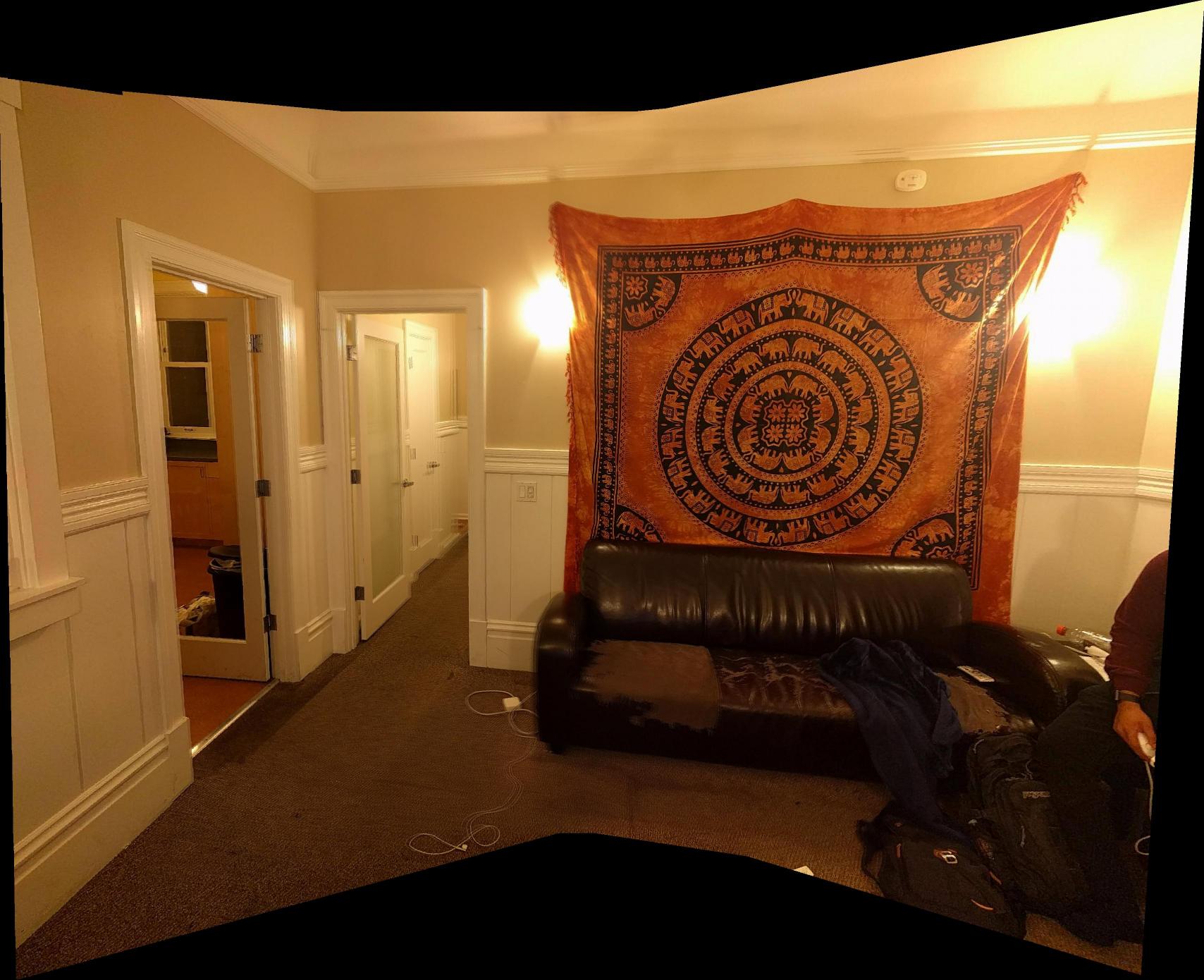
Mosaicing

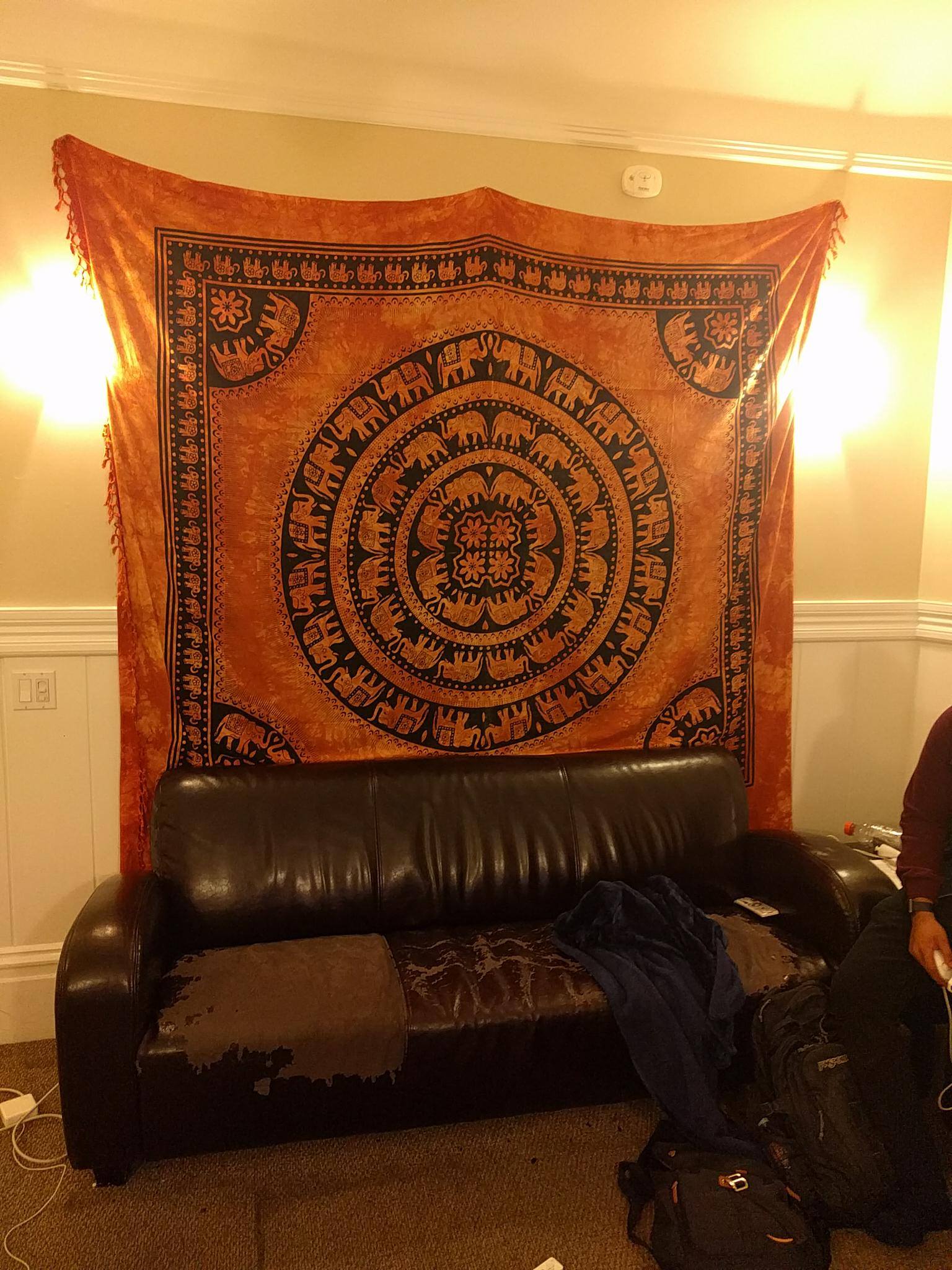
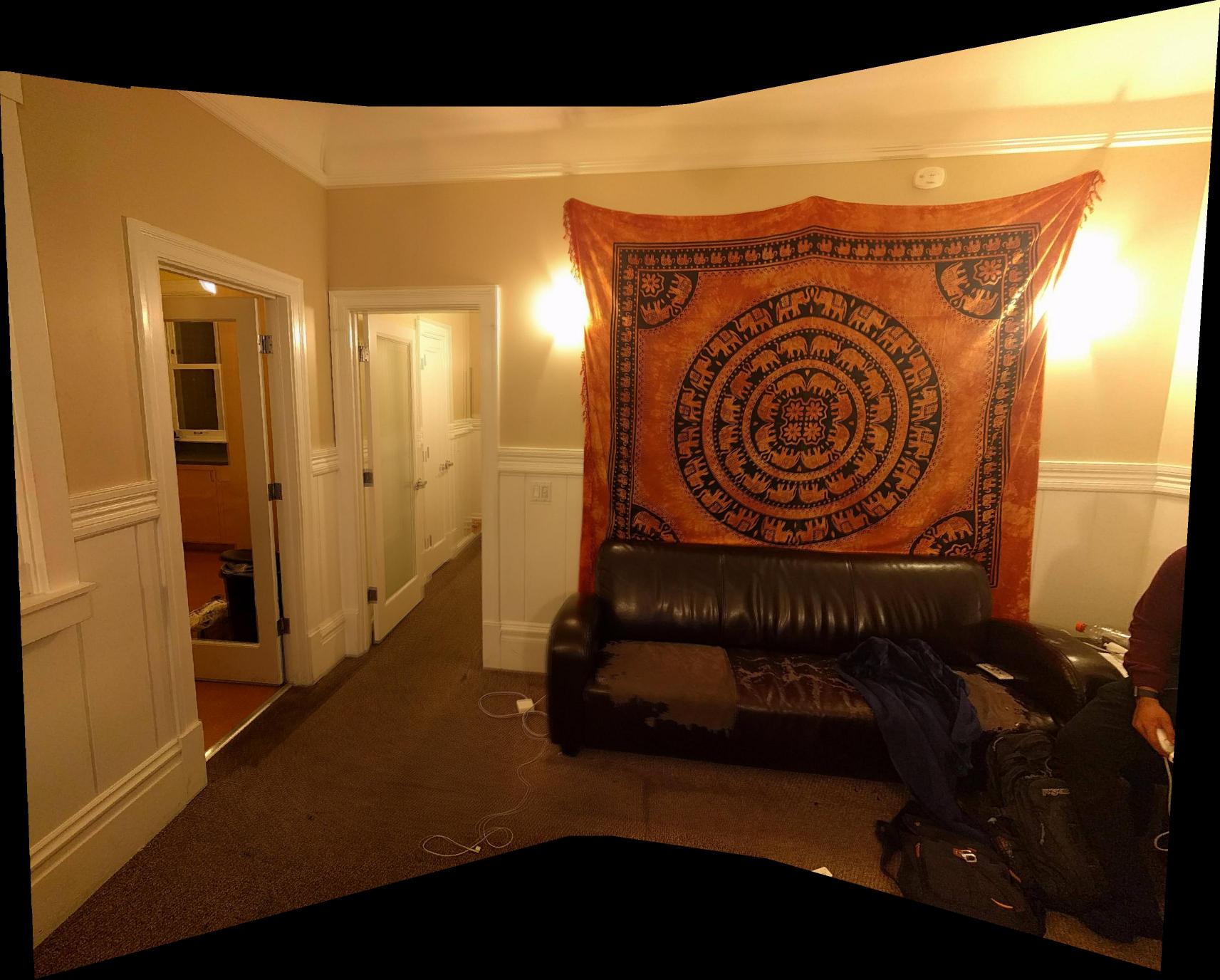
Here is the result of me putting together the first two images in my settings. There are a couple problems. First, there is a hard boundary between the two images. This will be more evident in the next section. Second, the image is blurry in areas. This is especially evident in the vertical lines on the tapestry.

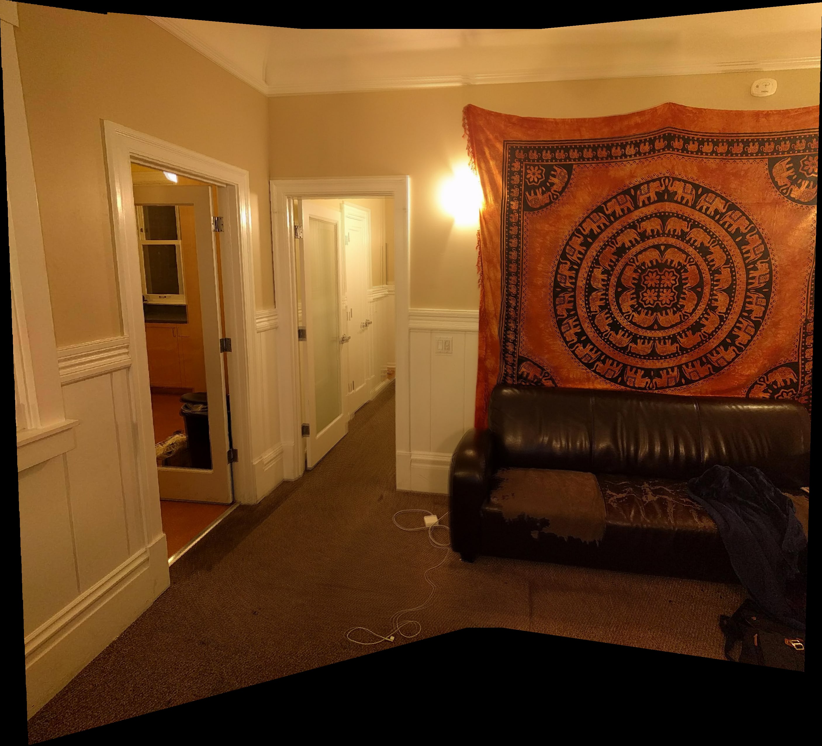
Weighted Averaging

Here, I do a weighted average. I chose to weight the pixel higher if its closer to its corresponding image's center. That way, theres a gradient from the left image to the right in the pixel weights. This helps with some of the blurriness, and gets rid of the lines between the borders of the images:

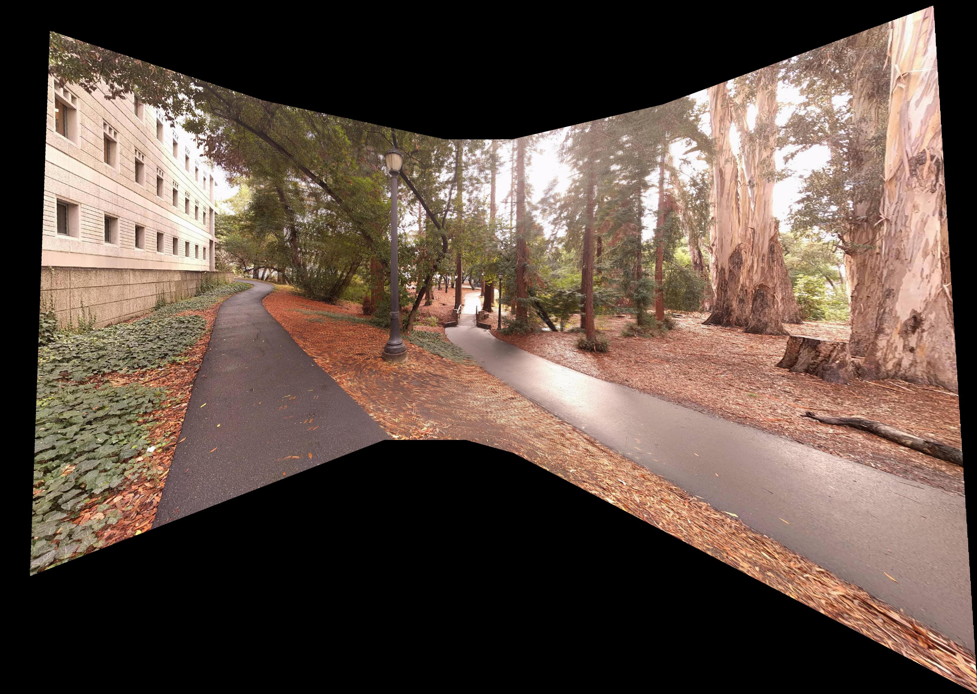
Final Results

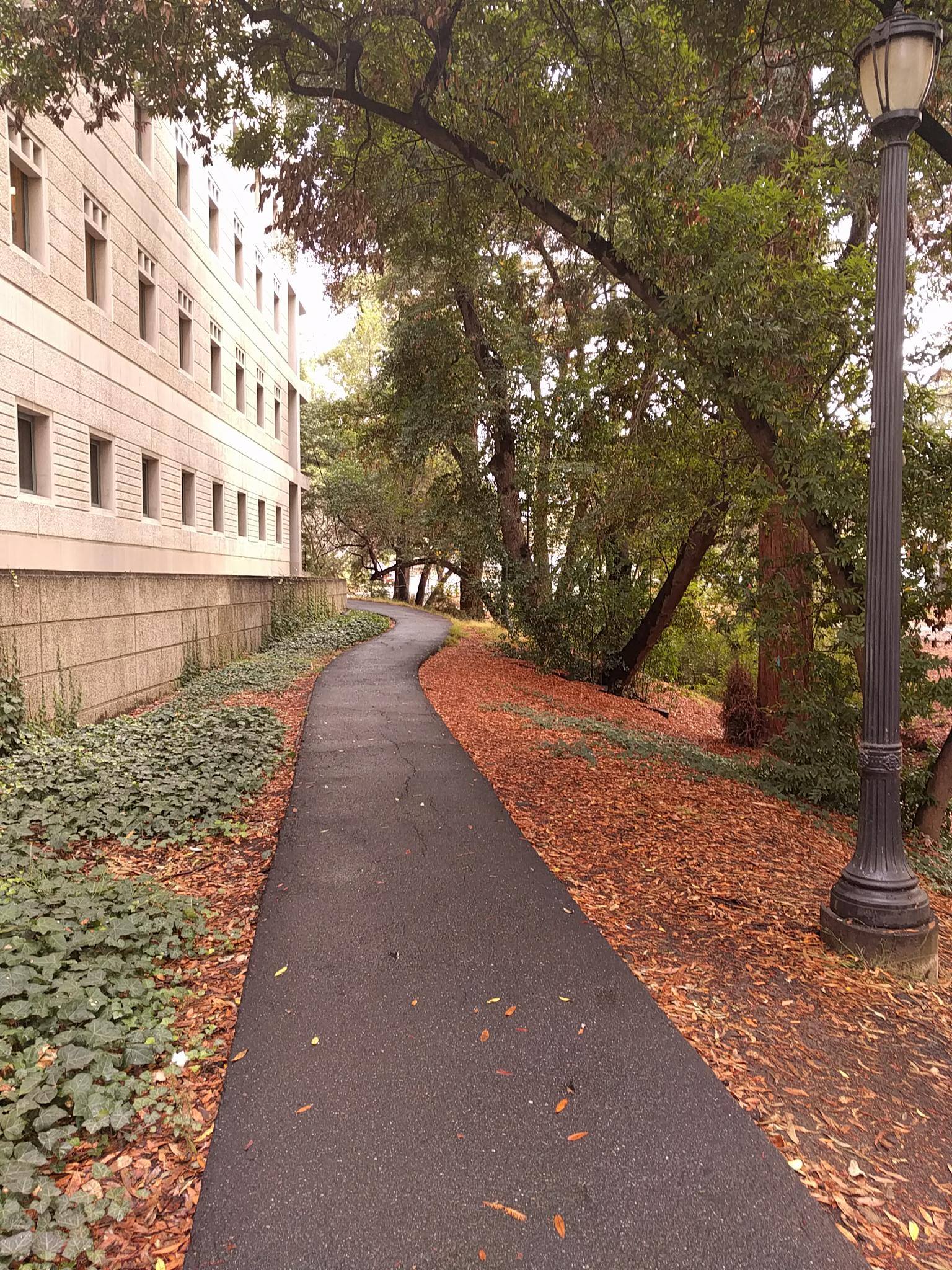
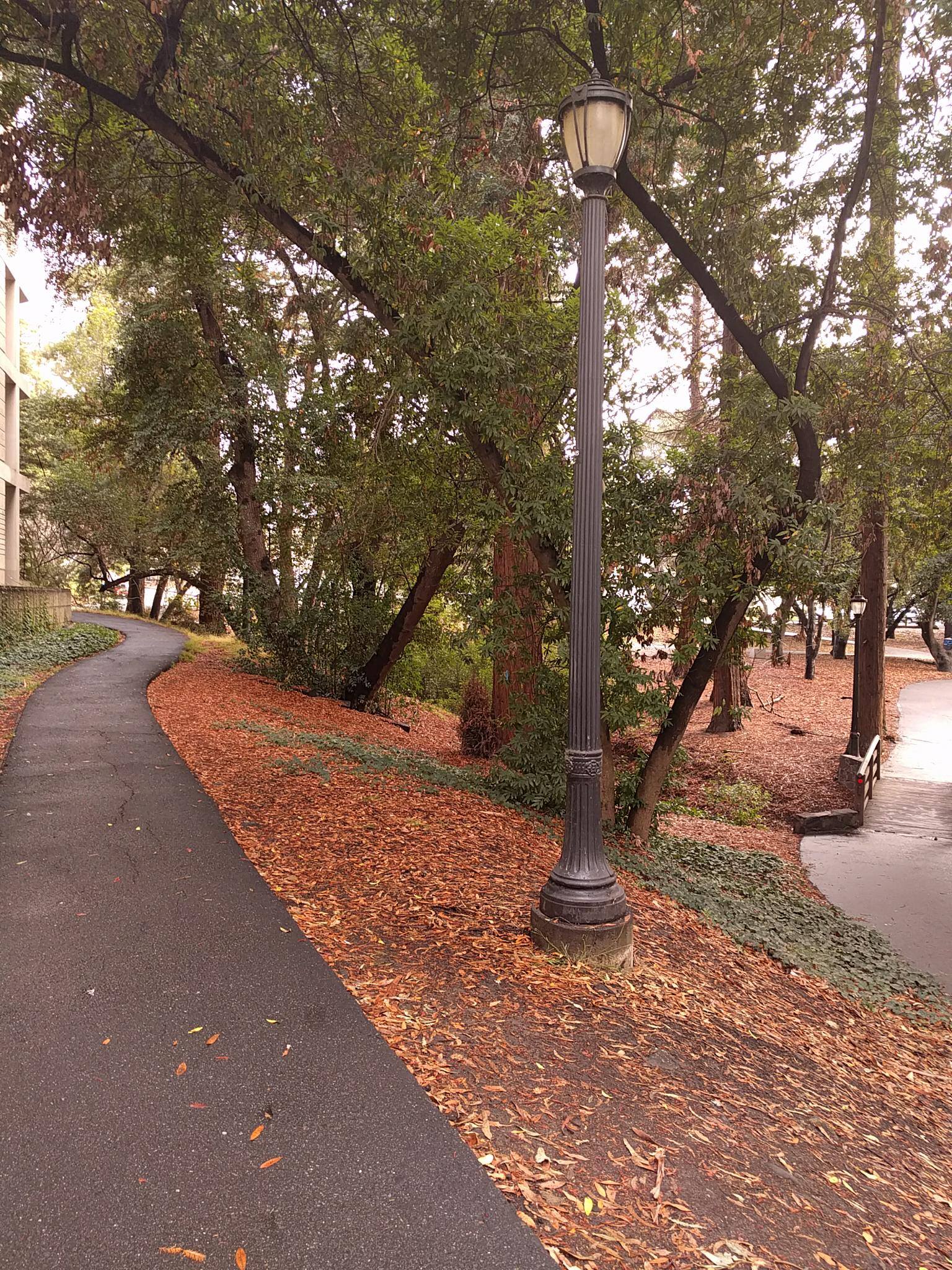
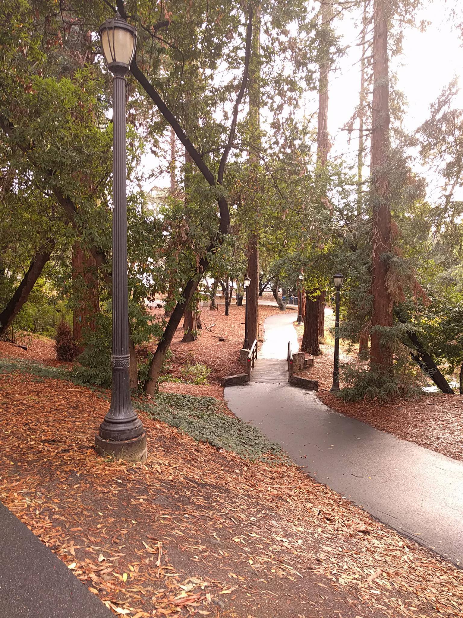
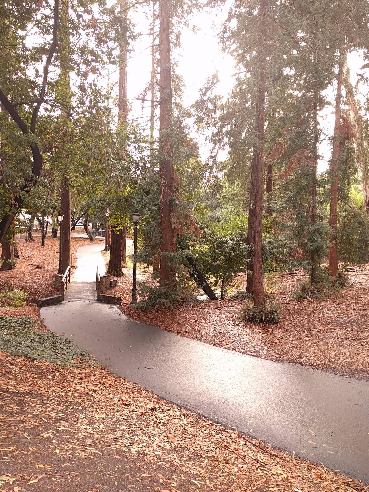
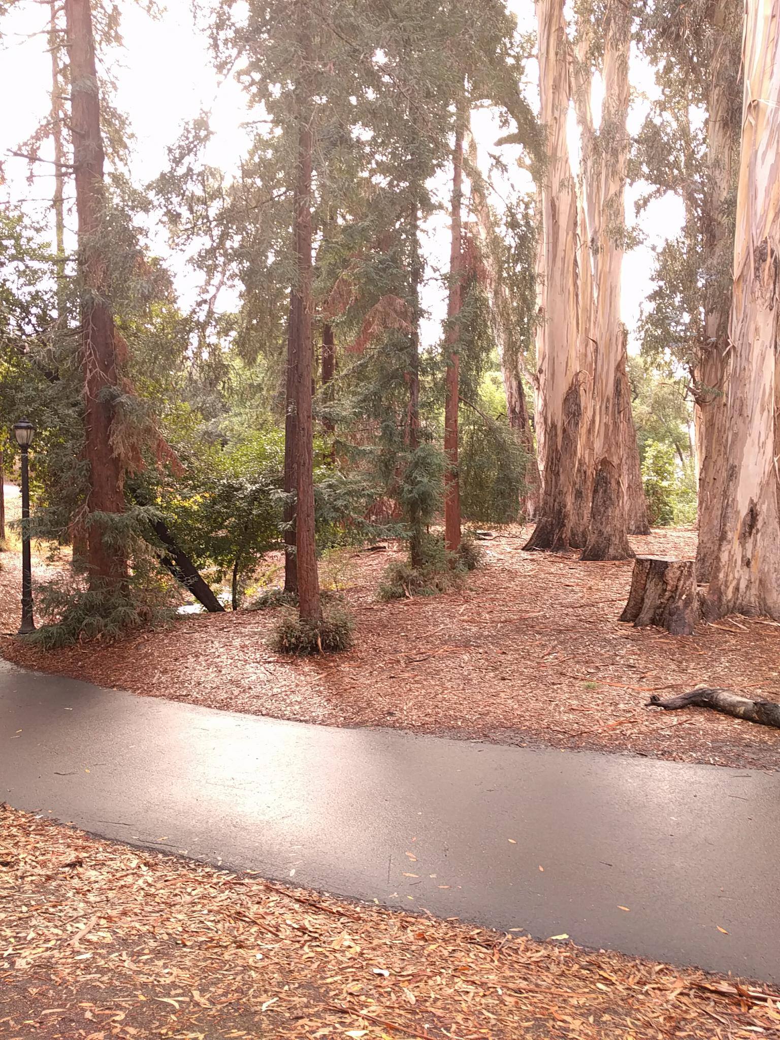
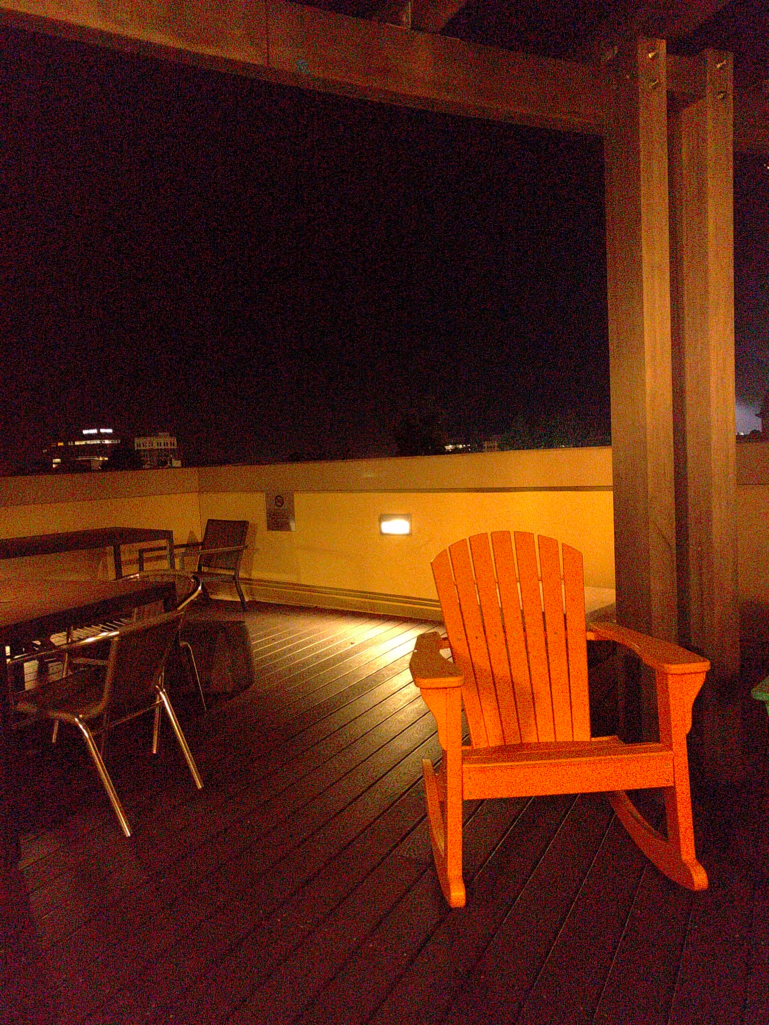
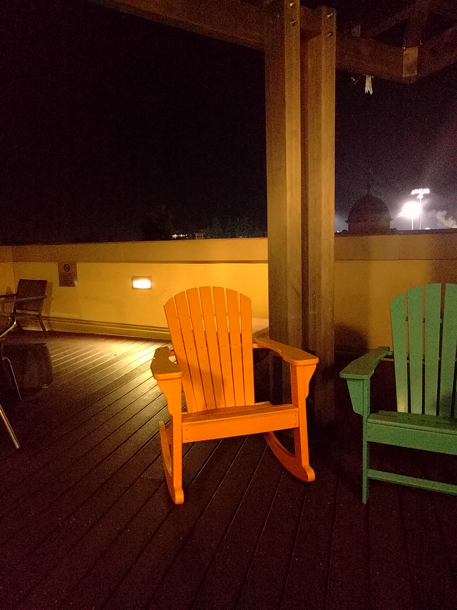
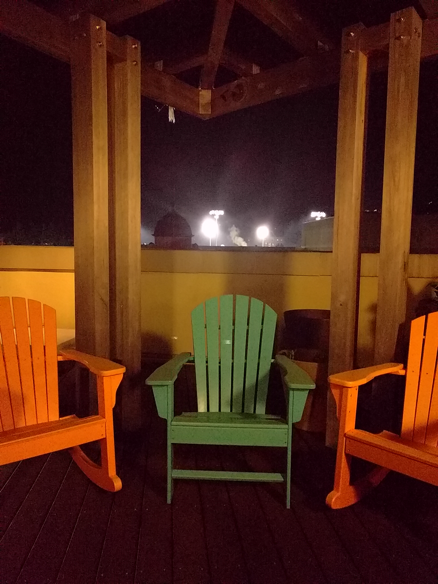
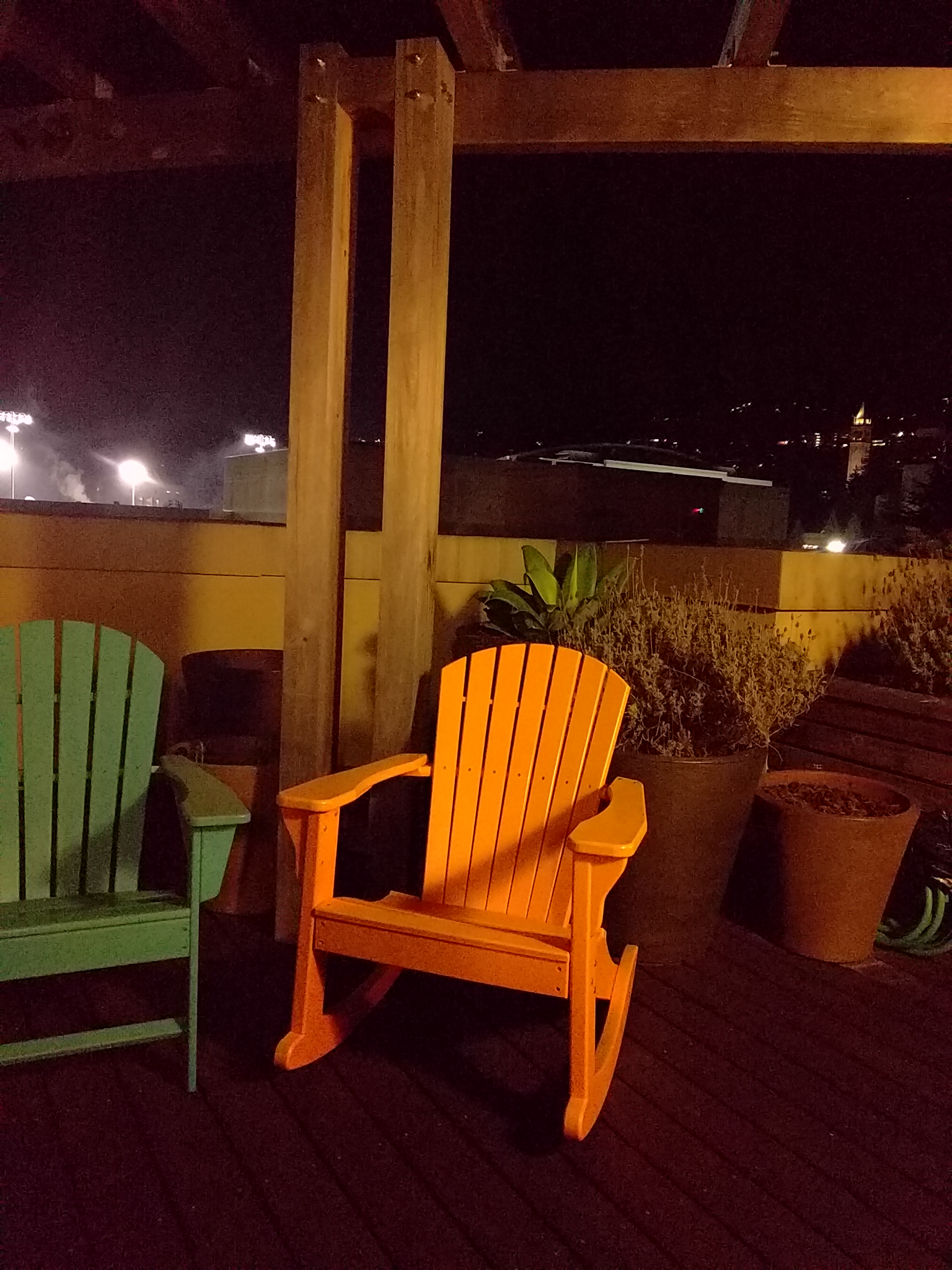
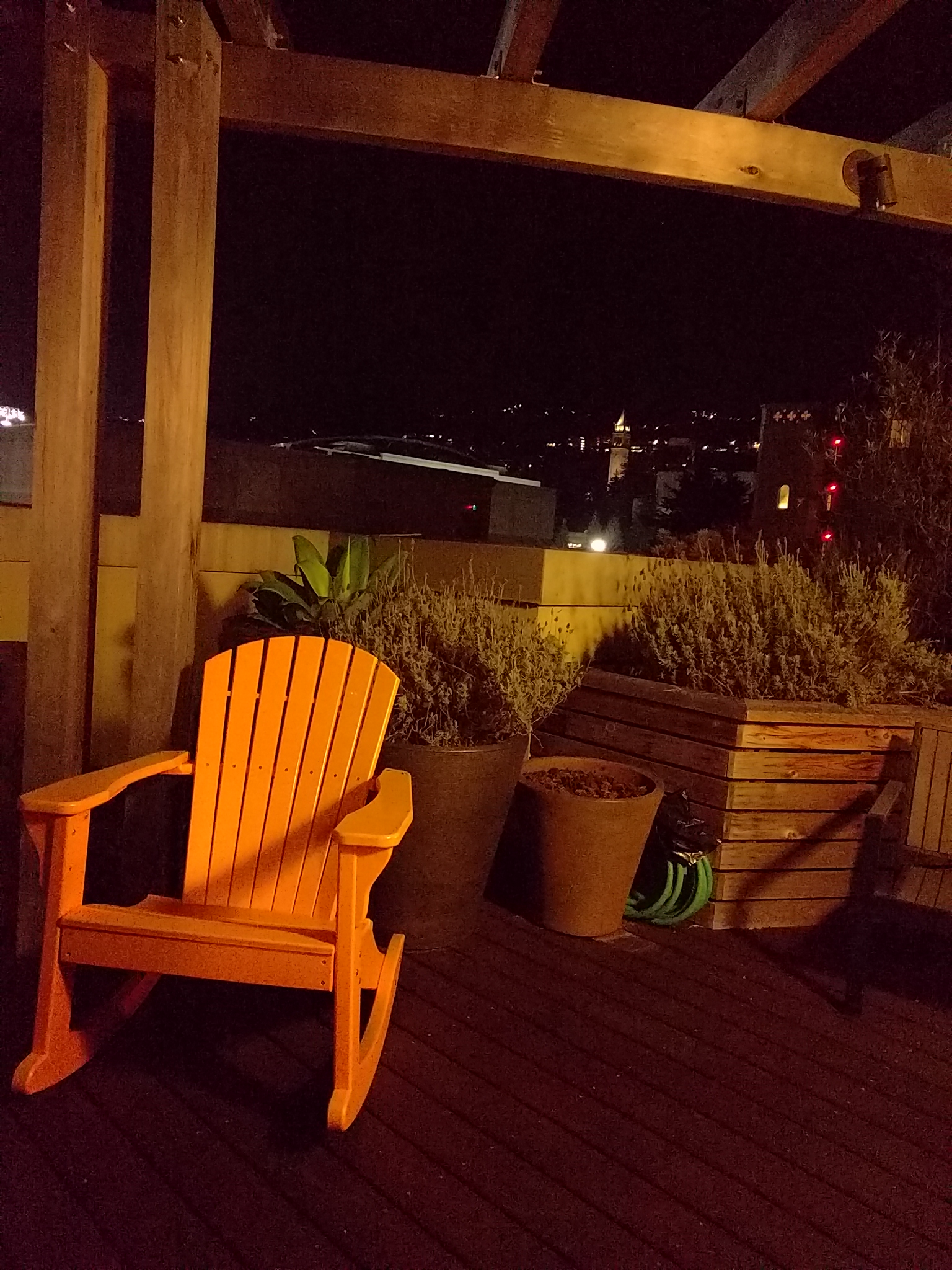
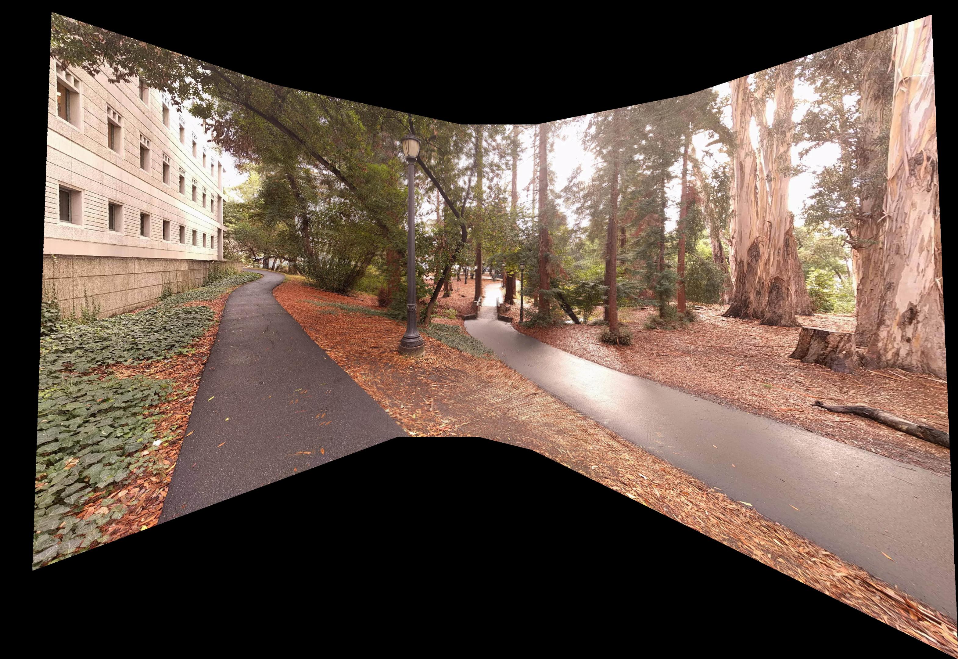
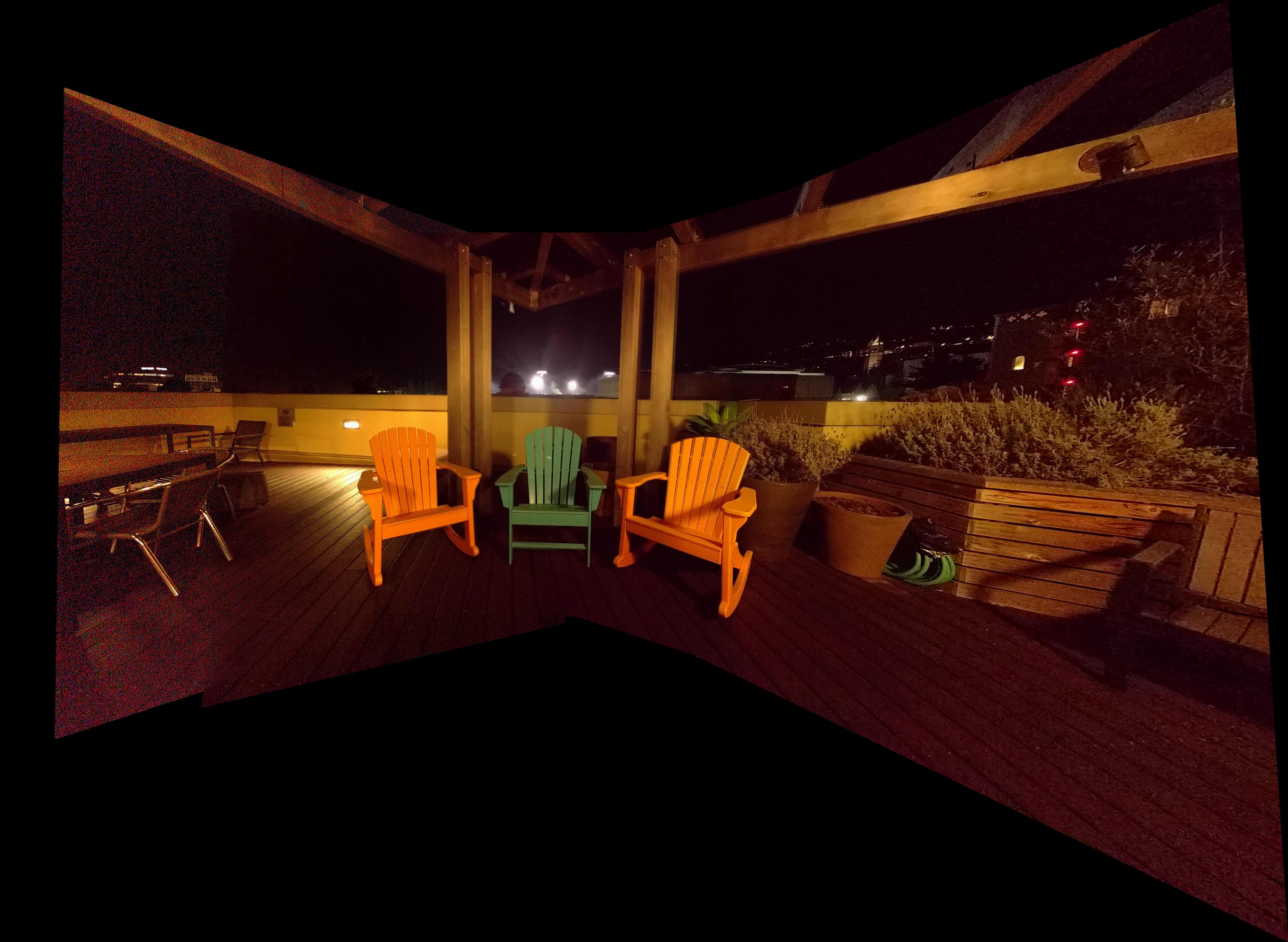
I took three full panoramas. The first was my apartment's living room. The second is one of my favorite spots on campus. The final panorama is of my friend's rooftop, off campus.

What I've Learned

From this project I ovbviously learned how to calculate homogrophies and blend images together. Beyond that, I found that found that the mosiacs are very sensitive to small changes between images. Even though I did a weighted average to blend the images together, you can see a difference between the leftmost image, and the second from the left. This is because I took the pictures at night, which meant I had to turn the ISO up a lot. the leftmost image was noisy, since there was little ambient light, but the second from the left got the city lights in the background, so it wasn't as noisy. The blending helped with the boundary, but you can still see a difference.

Second, I learned that choosing points is an art. I found that sometimes, selecting more points was not always better. If I selected many points, but in a small area, it would tend to find a homography that satisfied that one area better, sacrificing performance in other areas. By selecting fewer points, but more uniformly spread across the image, I was able to recover a much better homography.

PART 2

Harris Point Detection

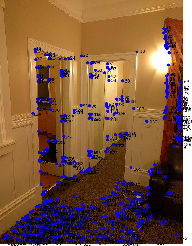
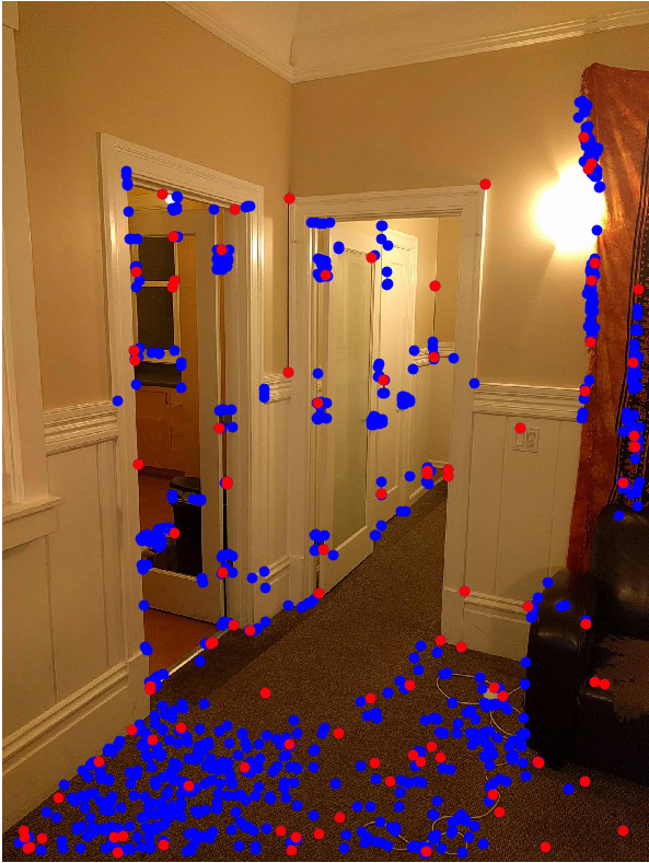
I ran the starter code to get the Harris points:

Adaptive Non-Maximal Suppression (ANMS)

The Harris Point Detection returns way too many points. We would like to take the points that correspond to the best "corners". However, we want the points to be fairly uniformly spread across the image. We use the ANMS algorithm to select a subset of the Harris points.

Intuitively, we would like to take the best corners in its surrounding area. For every point, we compute the distance to the closest "better" point:

  ri = minj|xi-xj|, s.t. f(xi) < crobustf(xj)
  

We then take the points which have the largest minimum distances. In the next image, the red points are the subset of the blue dots that were selected by ANMS:

Feature Descriptors

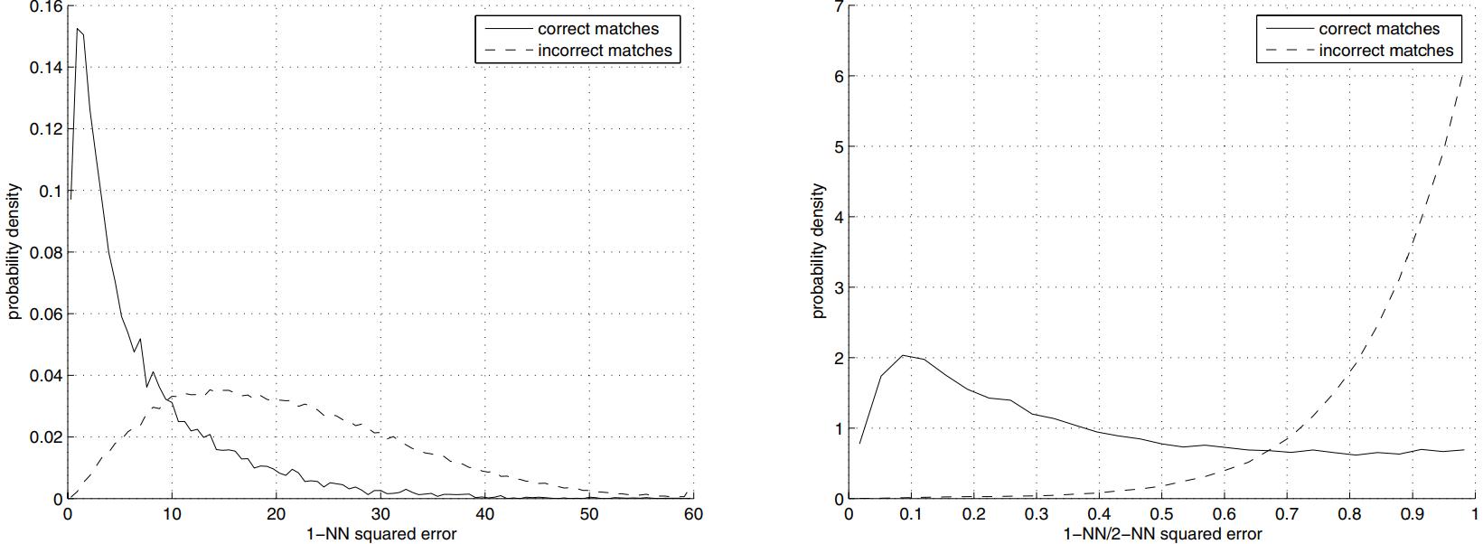
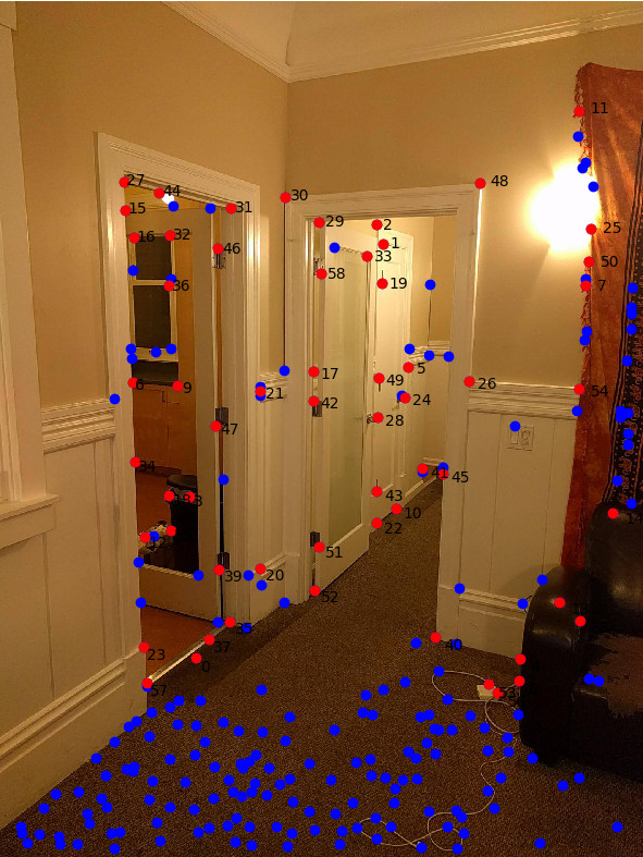
Feature Matching

Intuitively, we want to match each point to the nearest neighbor. However, it is sometimes hard to separate the good matches from the bad. To combat this, we use the Lowe ratio. For every corner's feature, we find the nearest neighbor in the second images corners, and the second nearest neighbor. I divide them to find the Lowe Ratio. In the following plots, you can see why the Lowe Ratio significantly separates the distributions of errors for the correct matches and incorrect matches. For each match, if the Lowe Ratio is below a certain threshold, we can be confident that it is a match. As you can see, there are a couple of mismatches, like point #1 and #6 on the left image.

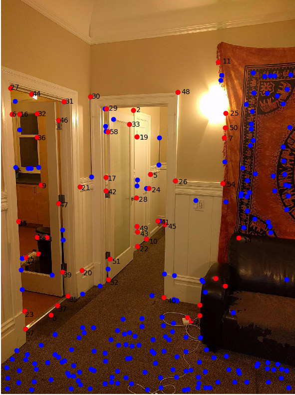
RANSAC

In case some points can still be false positive matches. We use the RANSAC algorithm to filter out any last outliers. To do this, we select 4 random matches, and create a Homography. From this homography, we compute the distance from each point to its corresponding point in the other image. If it is significantly different, it is assumed to be disagree with the 4 randomly selected points. We run this a couple of times, until we find a set of 4 randomly selected points that "agree" with the most points. In the following image, I plot the agreeing points in red, and the disagreeing (outlier) points in blue).

What I learned

In this part of the project, I learned how to automatically select correspondences. One unexpected thing I learned was related to the feature matching threshold. I originally selected a threshold of 0.4, in order to reduce the number of outliers. While, I got next to zero outliers, I later found that it was better to have a higher threshold, around 0.8, and have RANSAC remove the extra outliers. This is because the boundary of 0.4 would cut out many inliers while cutting out the outliers. Increasing the threshold allowed for many more points, and therefore much better stitches.

Auto Aligned Mosaics

Here are the results of the auto-stitched panoramas. As you can see, the results are slightly better than the hand selected counterparts. This is becuase it can be much more precise than me clicking points by hand.

Bells and Whistles: Panorama Recognition

In order to recognize panoramas, I ran my part 2 code on every pair of images. I set a threshold for the number of matching points. If the pair of images had more than the threshold of corresponding points, then I marked them as adjacent images. I then stitched the two images together, and then tried to match the stitched image with the remaining images.

I had to change my approach slightly. It would always attach the images in the correct order, but sometimes, it would warp the left image into the space of the middle image, and then warp the result in the space of the right image, rather than warping the right image into the space of the center image. The result would be a panorama that would not be centered around the subject.

I then modified my approach to check the number of adjacent images each image had, and merge images from the outside in. Here is the result of my living room, passing the images in the order: right, left, middle