// part a: image warping and mosaicing //
Image Rectification
We can take images and rectify them to a different plane; in other words, we can transform the image into a different plane as if we were viewing the scene from a different point of view. To do this, we take an image, pick at least four known points or "corners" on the image, and match those points into a shape of corresponding points that we expect these corners would look like in the new perspective's plane.
With the pairs of corresponding points, we compute the parameters of the homography transformation from the equation $p' = H * p$. The tranformation here is a homography with 8 degrees of freedom, or the 8 unknown parameters in $H$. However, after setting the scaling factor $i = 1$, there are only 7 remaining unknowns in the transformation matrix. Thus, for each pair of corresponding coordinates $(x, y)$ and $(x', y')$, we have:
$$
\begin{bmatrix}
wx' \\
wy' \\
w
\end{bmatrix}
=
\begin{bmatrix}
a & b & c \\
d & e & f \\
g & h & 1 \\
\end{bmatrix}
*
\begin{bmatrix}
x \\
y \\
1
\end{bmatrix}
$$
where $w$ is a scalar factor.
In order to solve for the parameters in $H$, we can first solve the above matrix multiplication as linear equations to eliminate $w$ from the equation. After doing so, we can set the new linear equations up as matrix multiplications of the form $A * h = b$, and end up with this system of linear equations per pair of corresponding points $(x, y)$ and $(x', y')$:
$$
\begin{bmatrix}
x & y & 1 & 0 & 0 & 0 & -xx' & -yx' \\
0 & 0 & 0 & x & y & 1 & -xy' & -yy' \\
\end{bmatrix}
*
\begin{bmatrix}
a \\
b \\
c \\
d \\
e \\
f \\
g \\
h \\
\end{bmatrix}
=
\begin{bmatrix}
x' \\
y' \\
\end{bmatrix}
$$
We add two more rows to $A$ and $b$ per pair of corresponding points. Once we've set the system of equations up, we can use the least squares solver to find the 7 missing parameters. After plugging our newfound values of $h$ into our transformation matrix $H$, we can use the homography transformation matrix with inverse warping to map every coordinate $p$ in an image to its corresponding coordinate $p'$ in the warped image.
Below, we have a gallery of images that are rectified to a frontal-parallel perspective. For each image, we've selected four points to match with what we expect to be in the shape of a square in the rectified image.
berlin street art
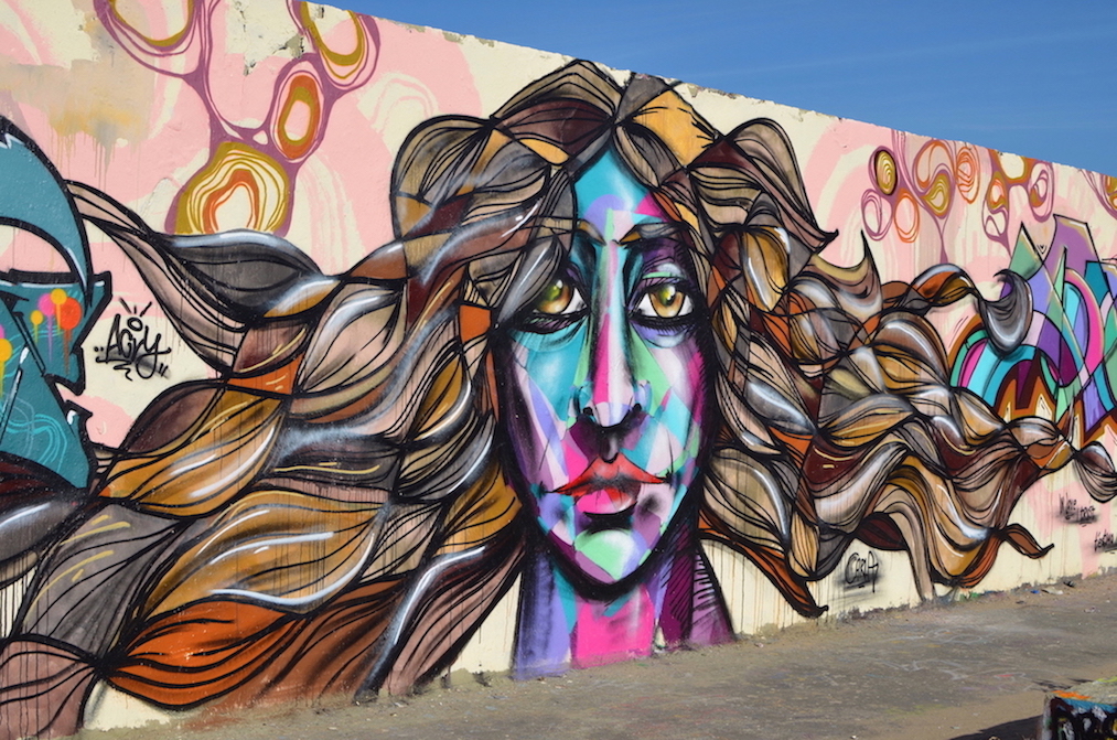
original view from left angle of the wall

rectified view from the center of the wall
details on a european church (i think)
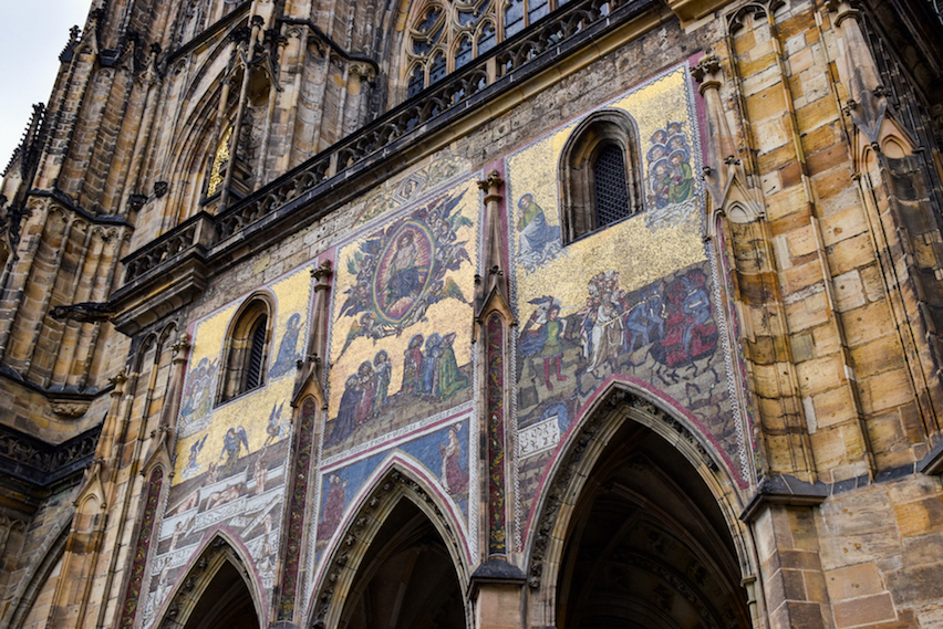
original view from left bottom right view of the building
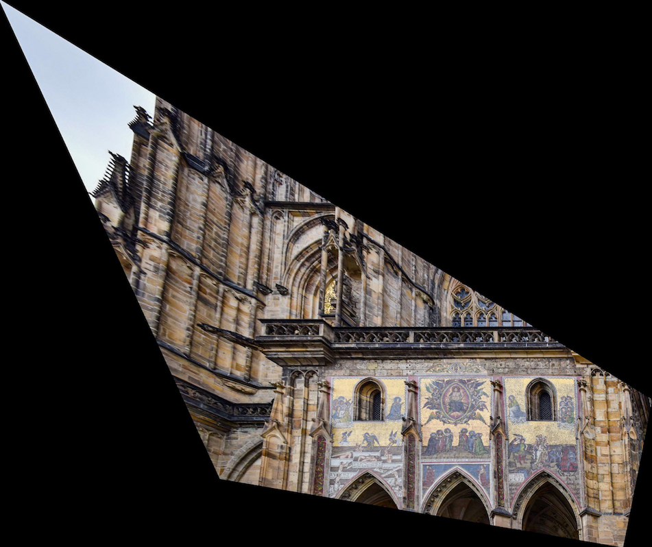
rectified view from the center of the building
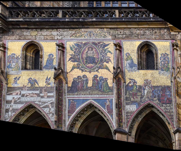
close-up of rectified view
berlin flea market table
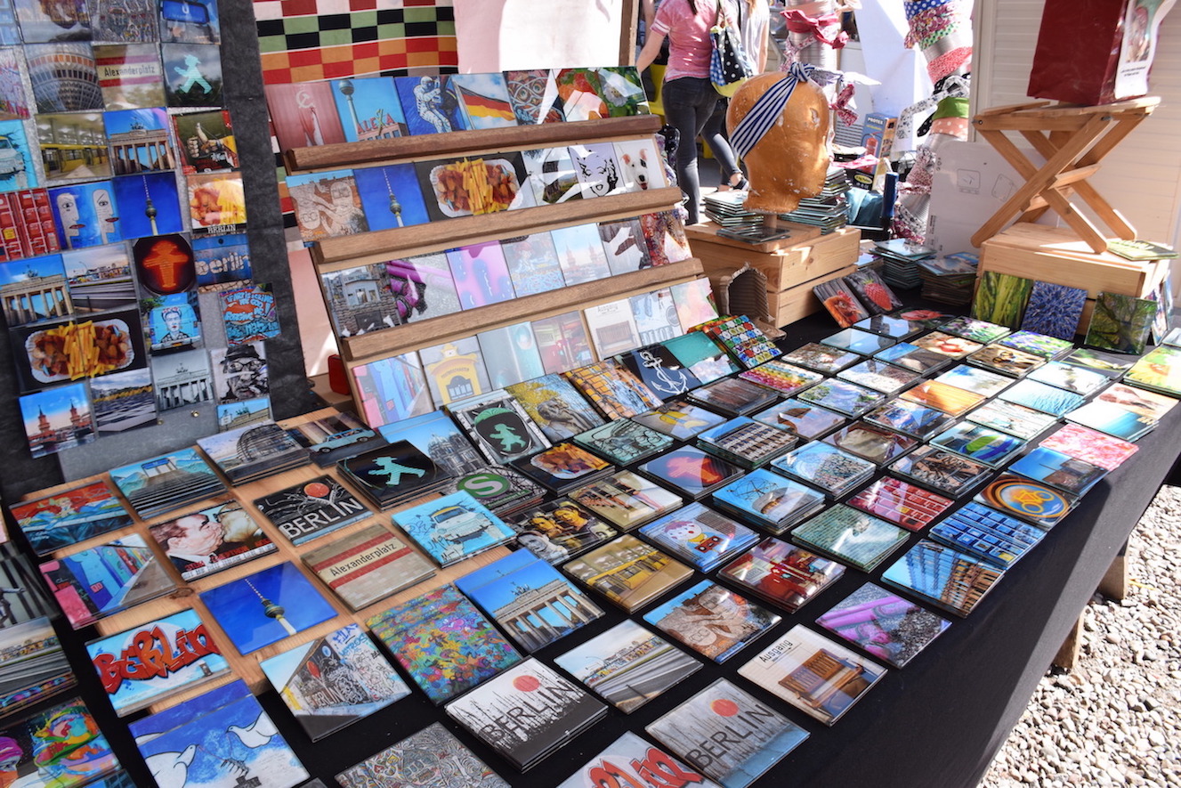
original view from left bottom side view of the table
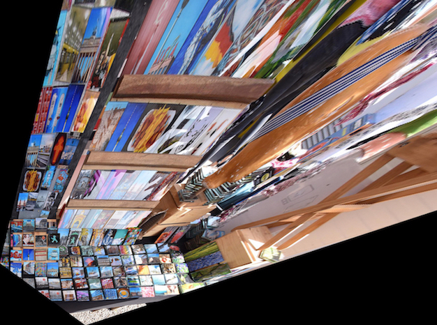
rectified view to the square board on the table (cropped for better view)

close-up of rectified view
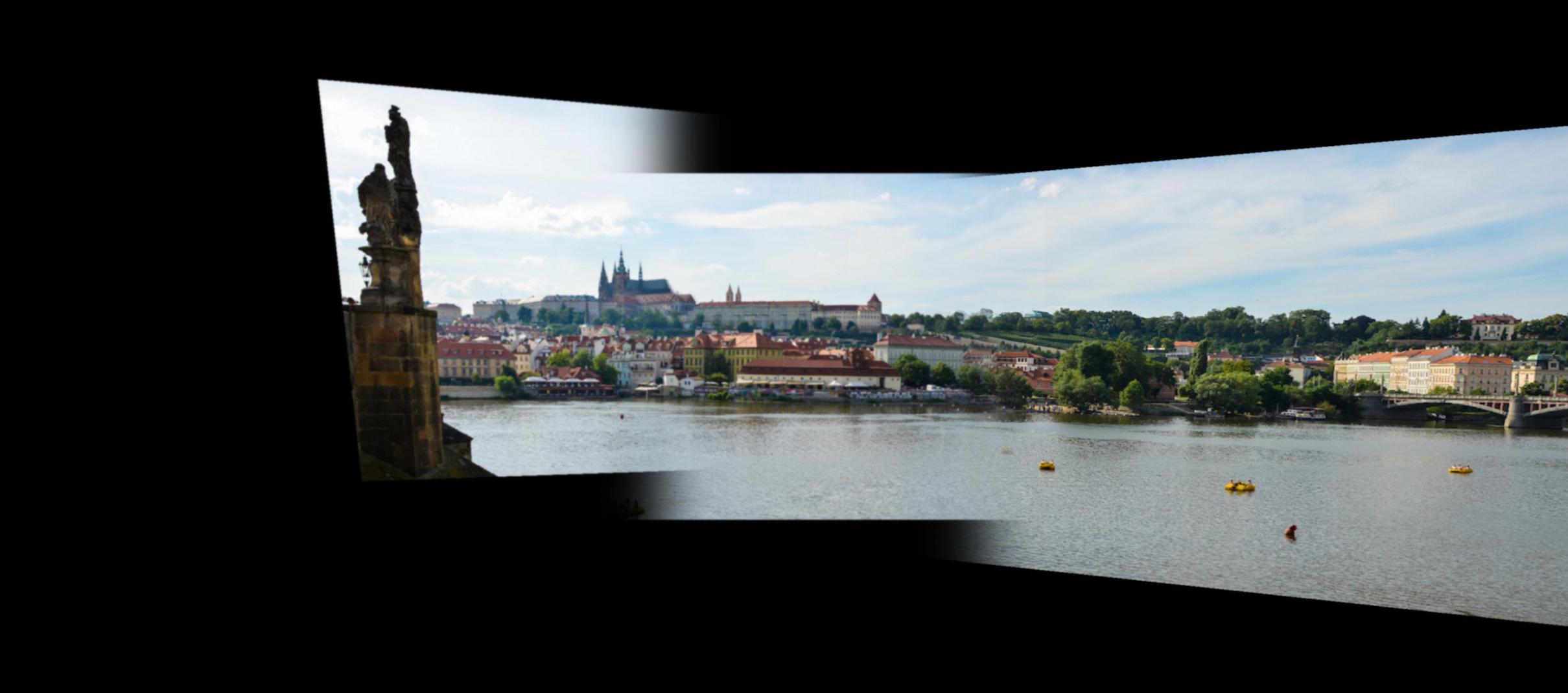
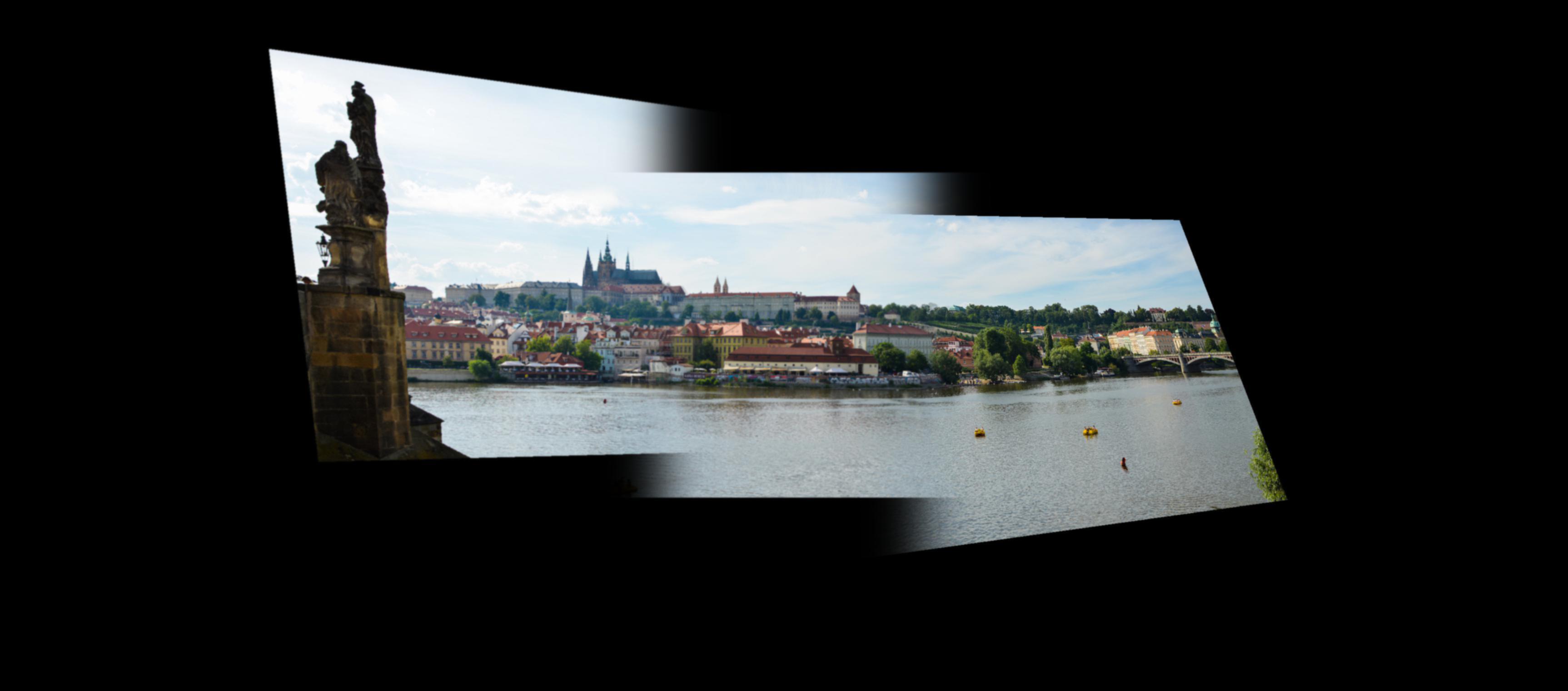
Mosaic Blending
Using the same idea from the rectifications above, we can also warp overlapping images with a projective transformation into the same plane and stitch the overlapping portions together so that they form a panoramic photo. First, we pick an image from the set to use as our static plane. Then, we pick corresponding points between the other photo(s) and the static photo, and again rectify the other photo(s) to the first photo we are using as our base. The rectification process again follows the same idea as rectifying it to a known shape--this time, the known shape is the points we chose on the static photo. Thus, we set up our transformation matrix and find the parameters of the homography transformation, then use inverse warping to create our new warped image. After getting these warped images, we use multiresolution blending/Laplacian stack blending (Project 3) to stitch the photos together along the seam of the overlapping regions.
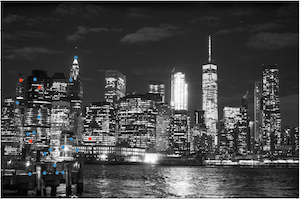
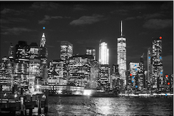
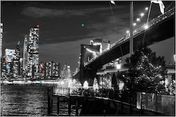
new york city skyline
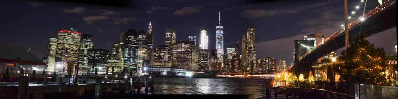
NYC skyline mosaic: cropped
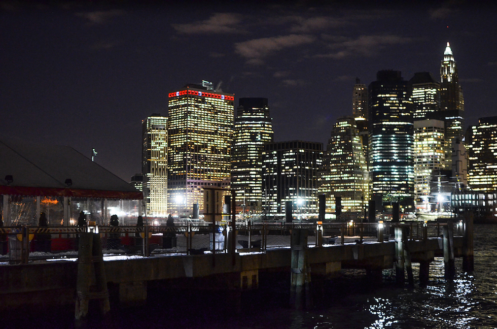
NYC skyline (left)
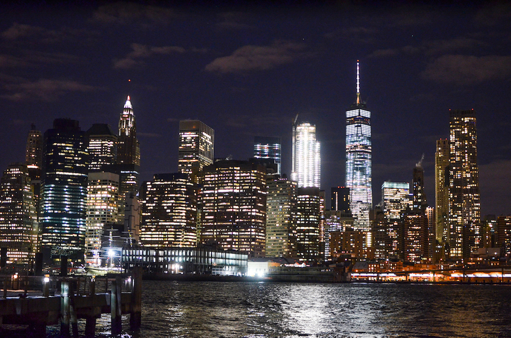
NYC skyline (center)
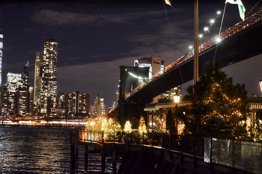
NYC skyline (right)
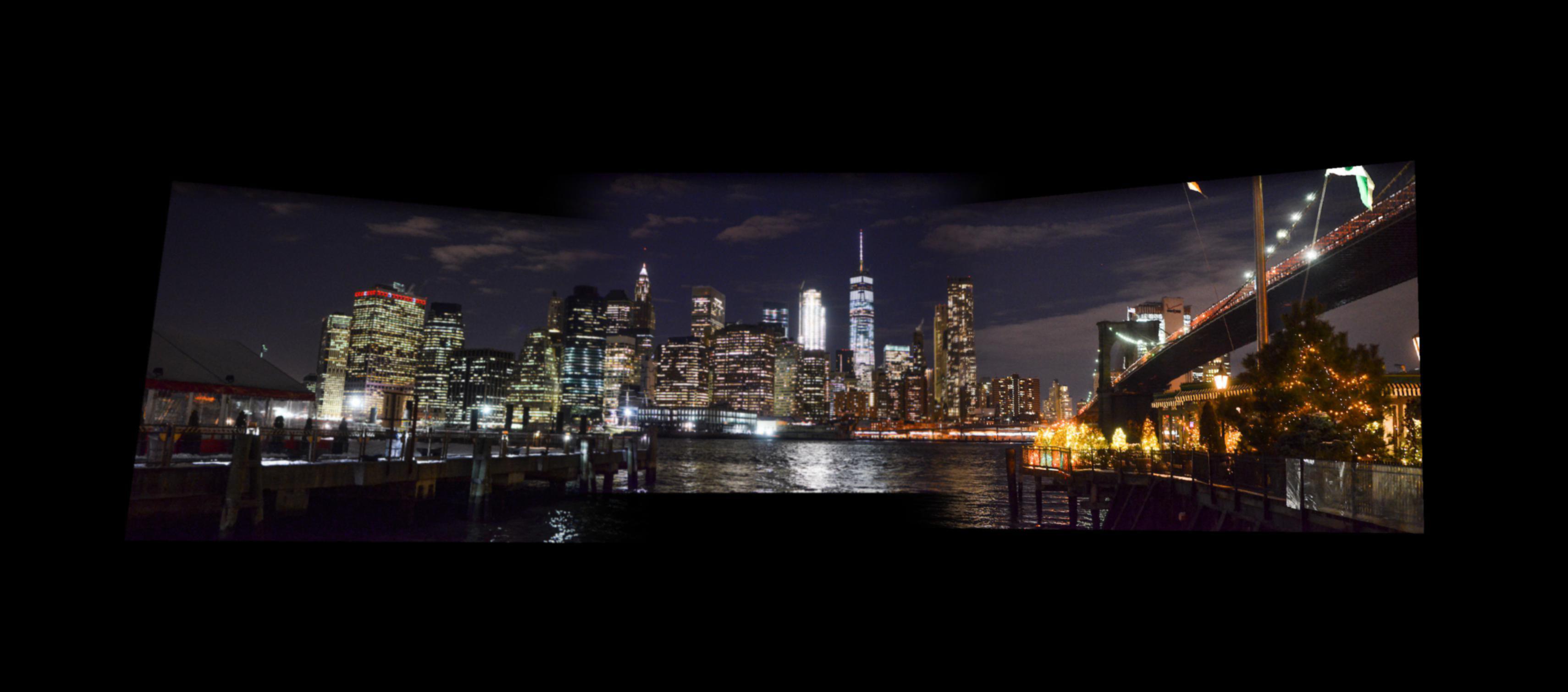
NYC skyline mosaic
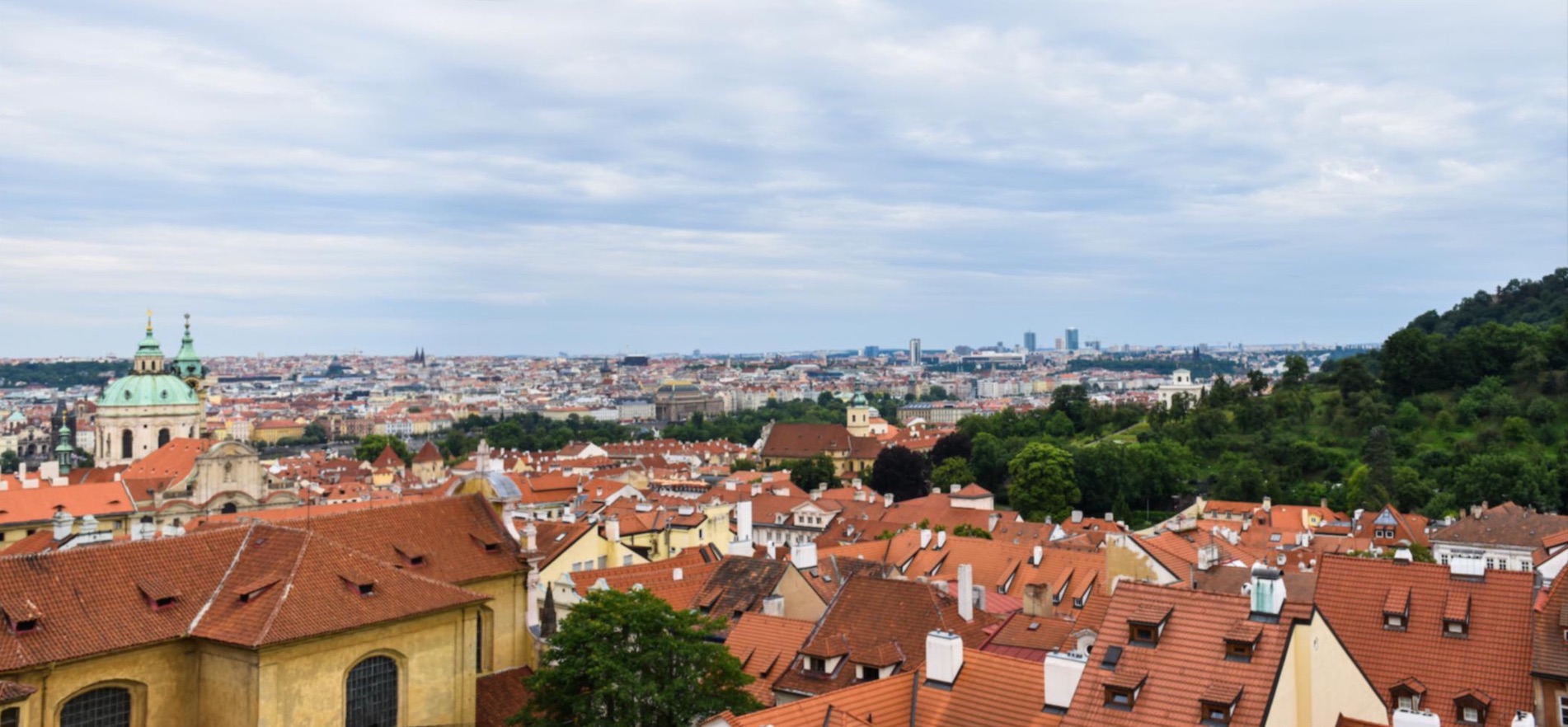
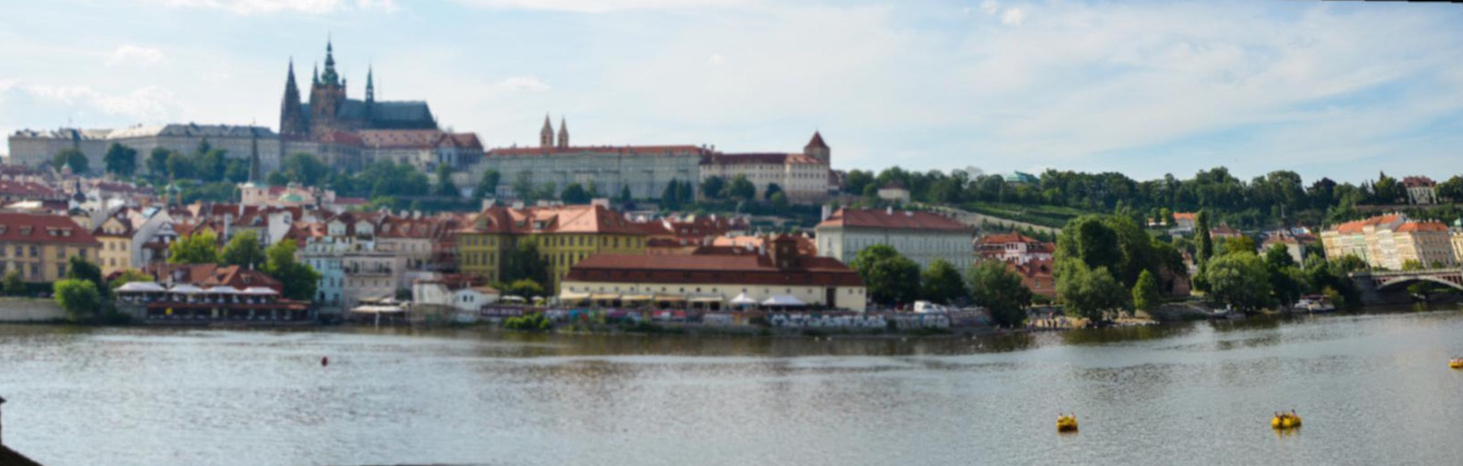
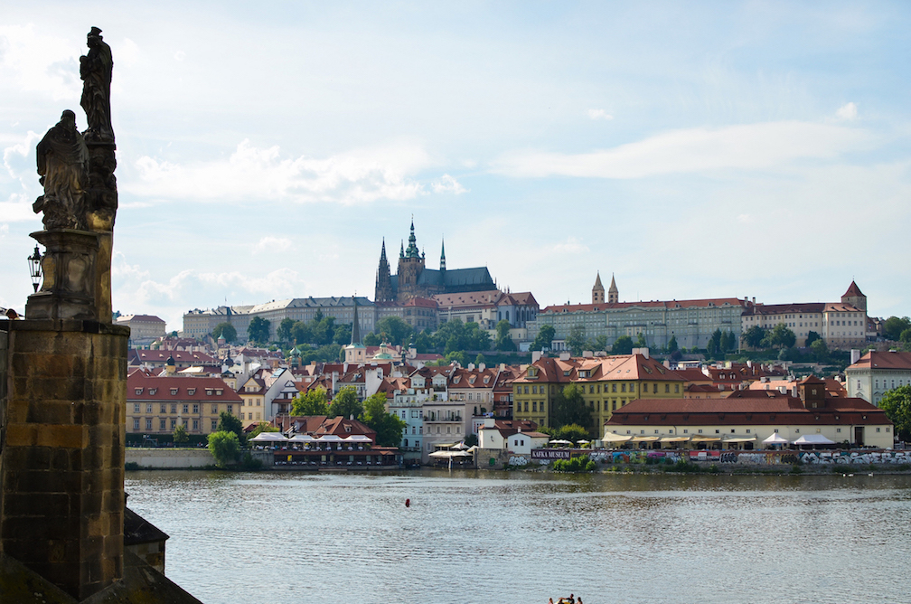
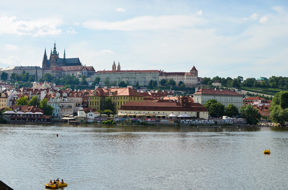
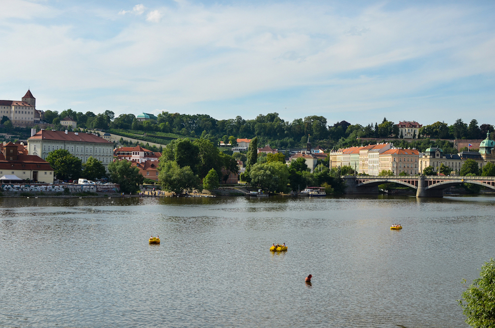
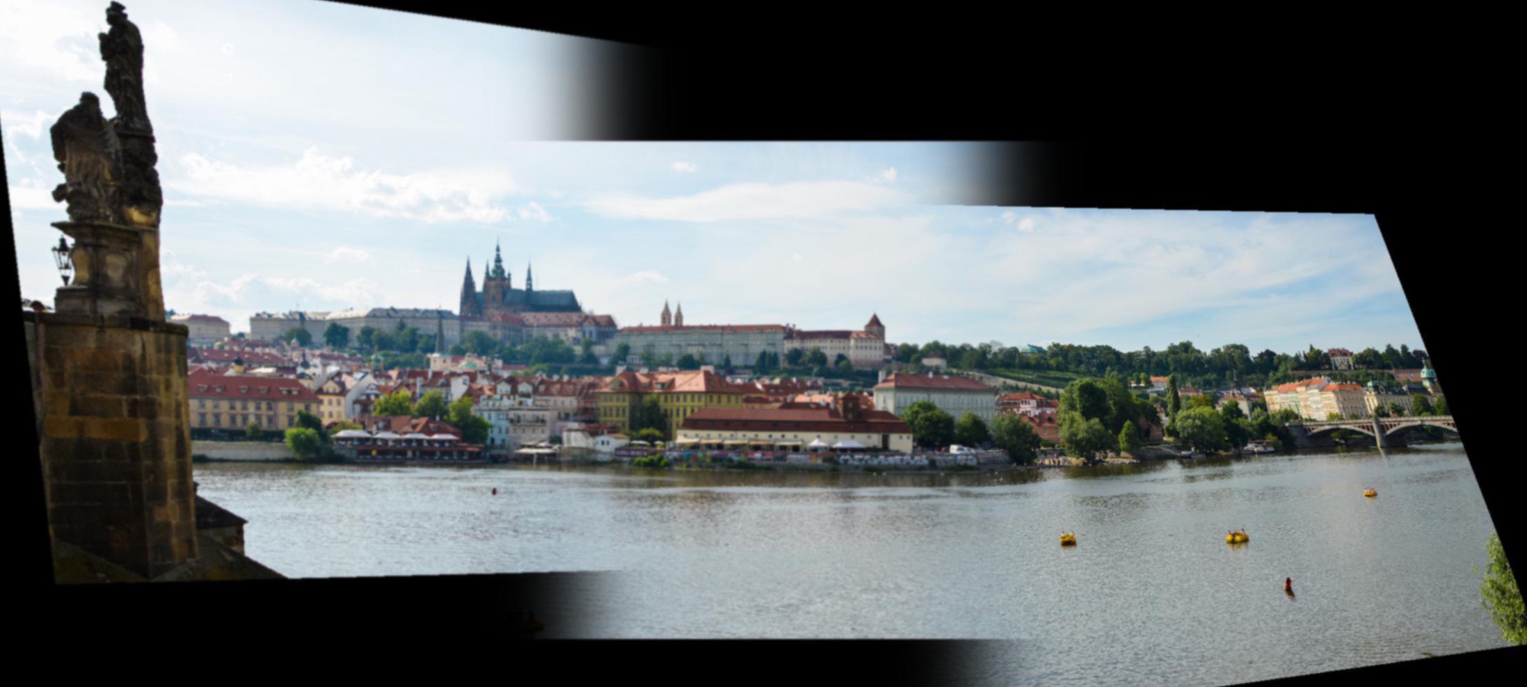
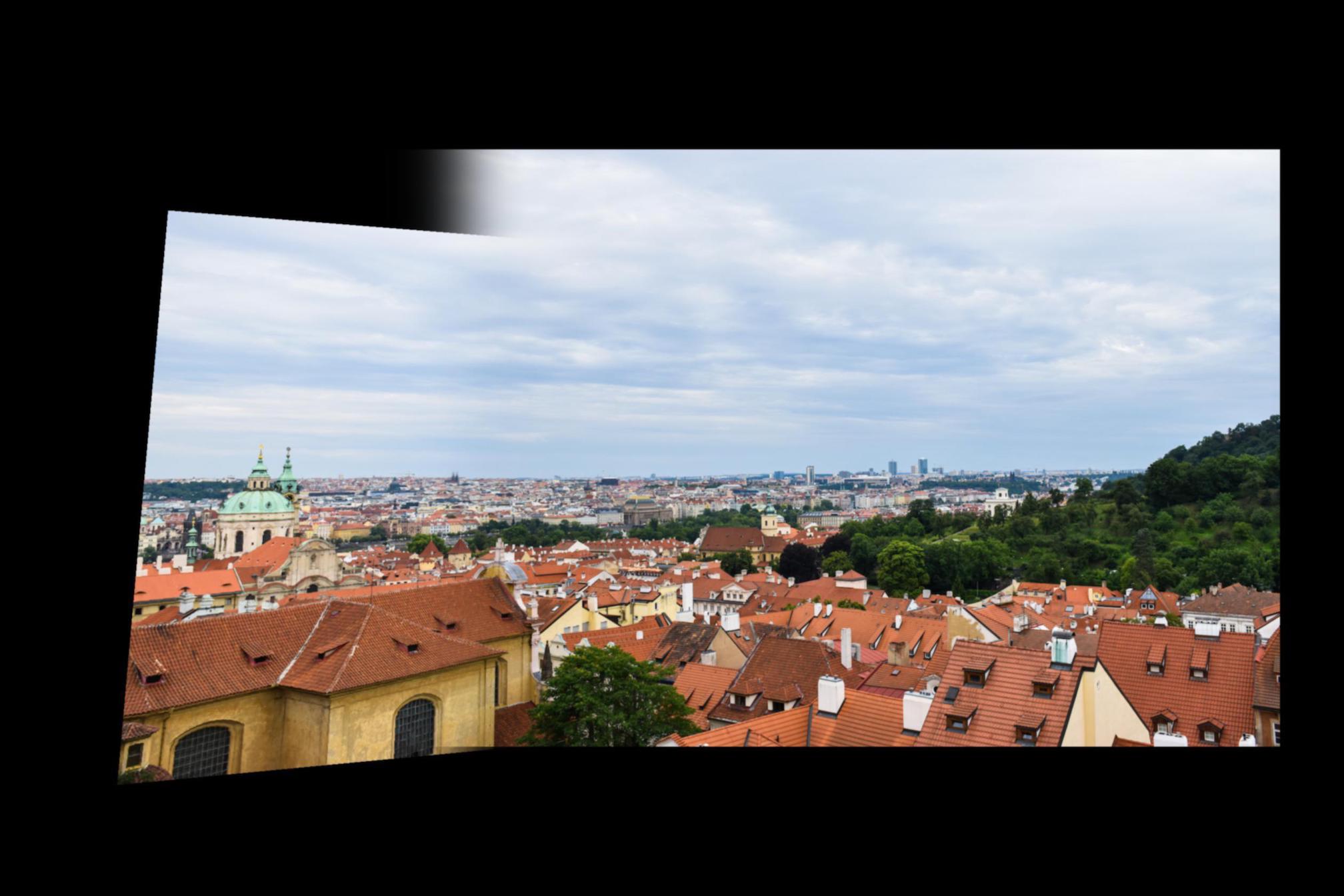
overlooking prague
prague mosaic: cropped
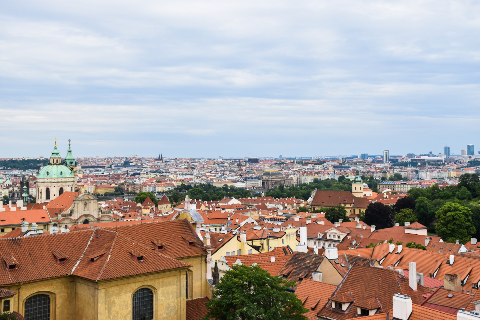
prague (left)
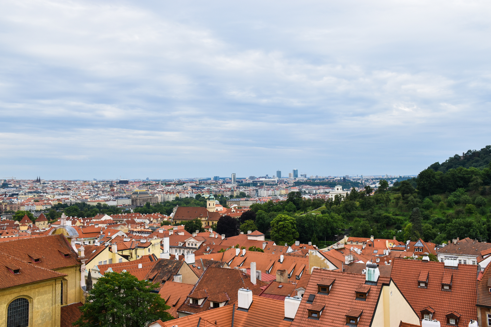
prague (center)
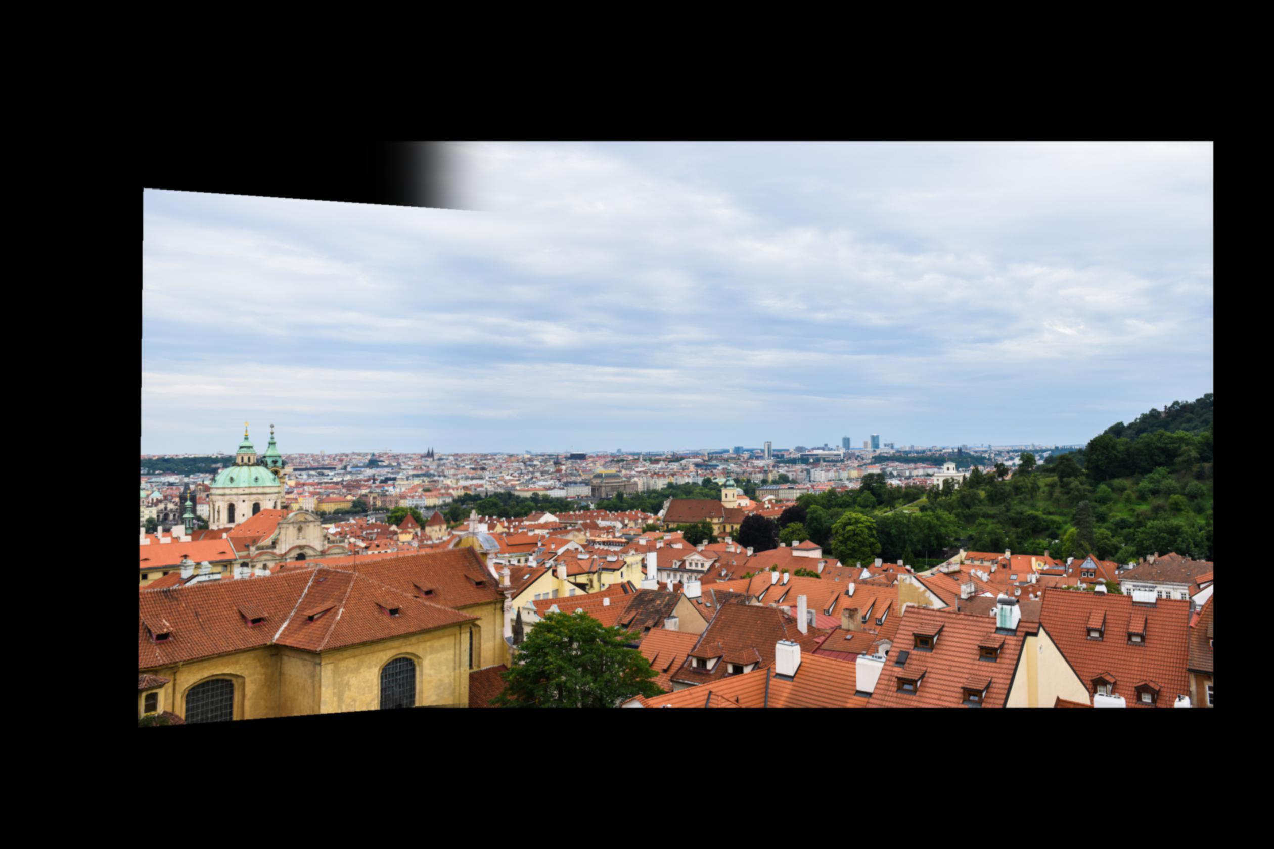
prague mosaic
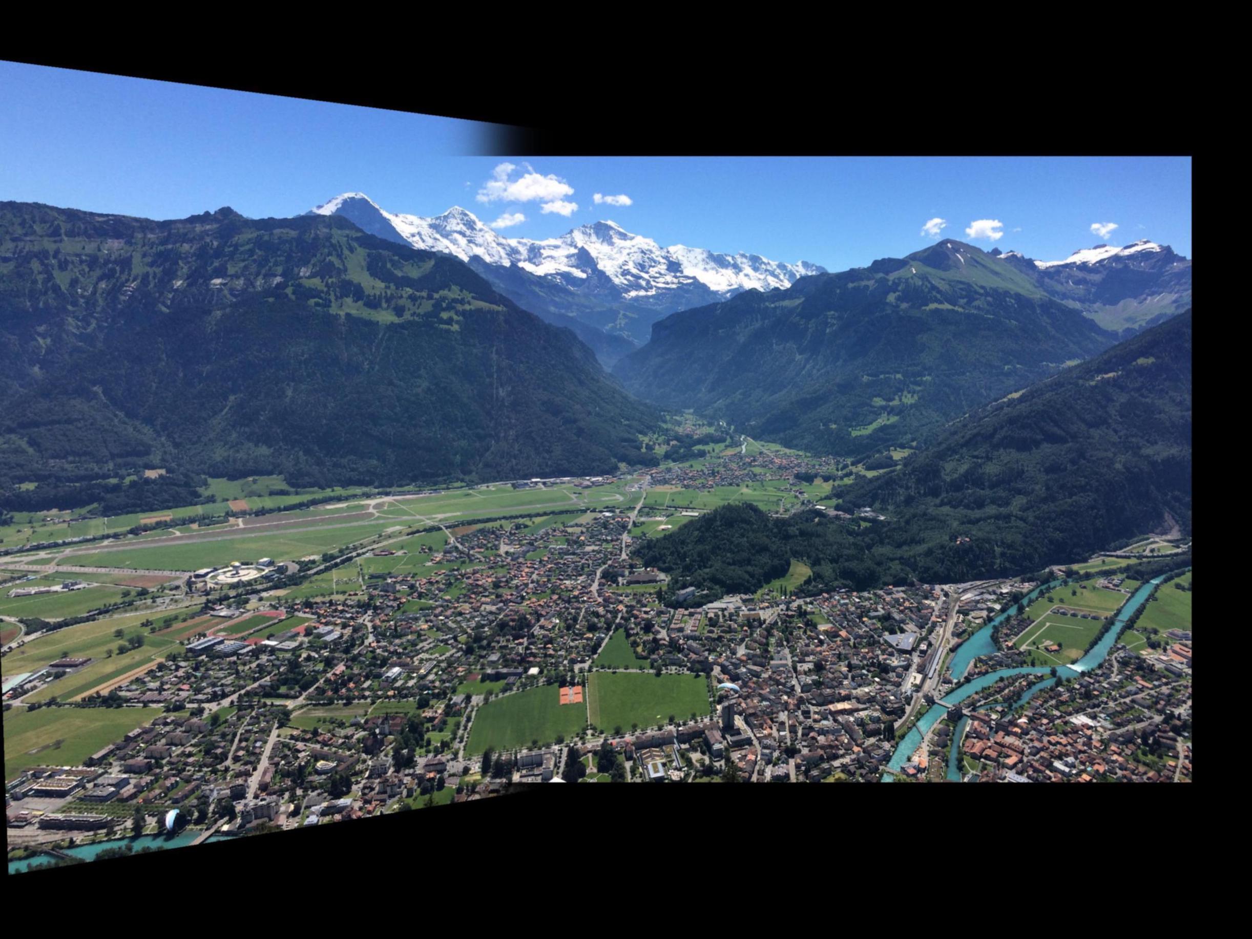
surrounded by the swiss alps
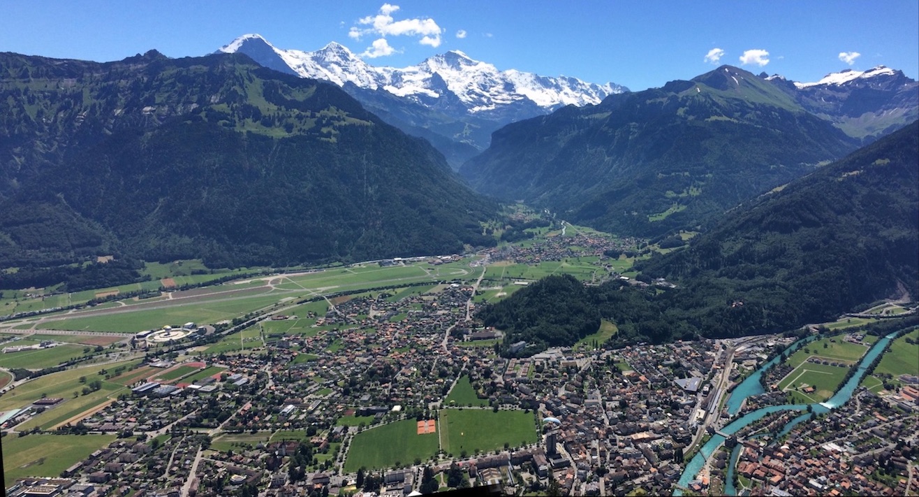
swiss alps mosaic: cropped
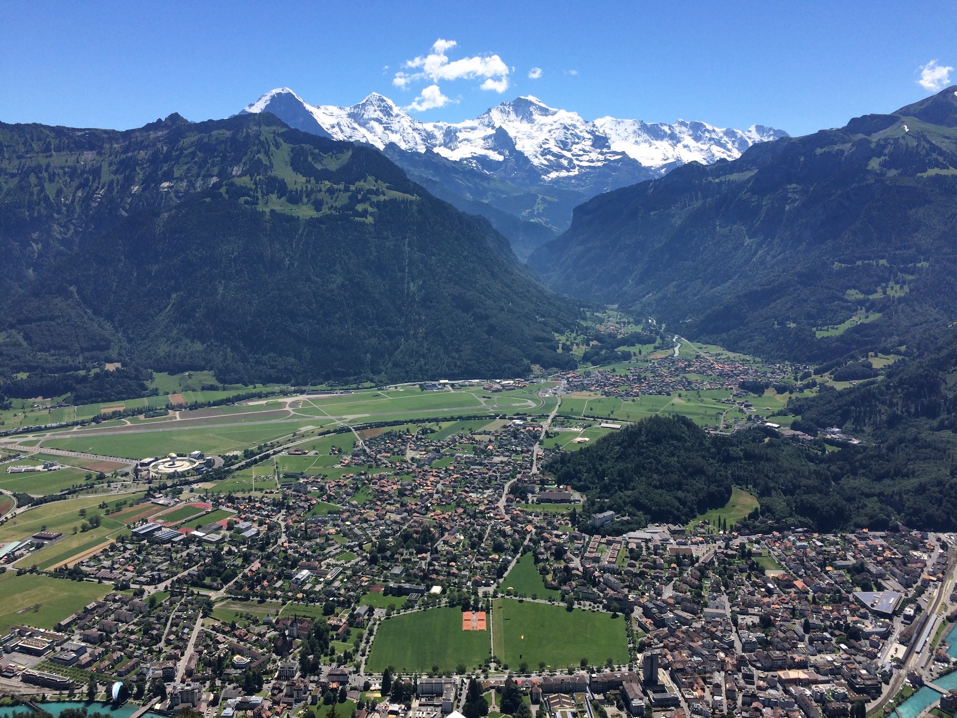
swiss alps (left)
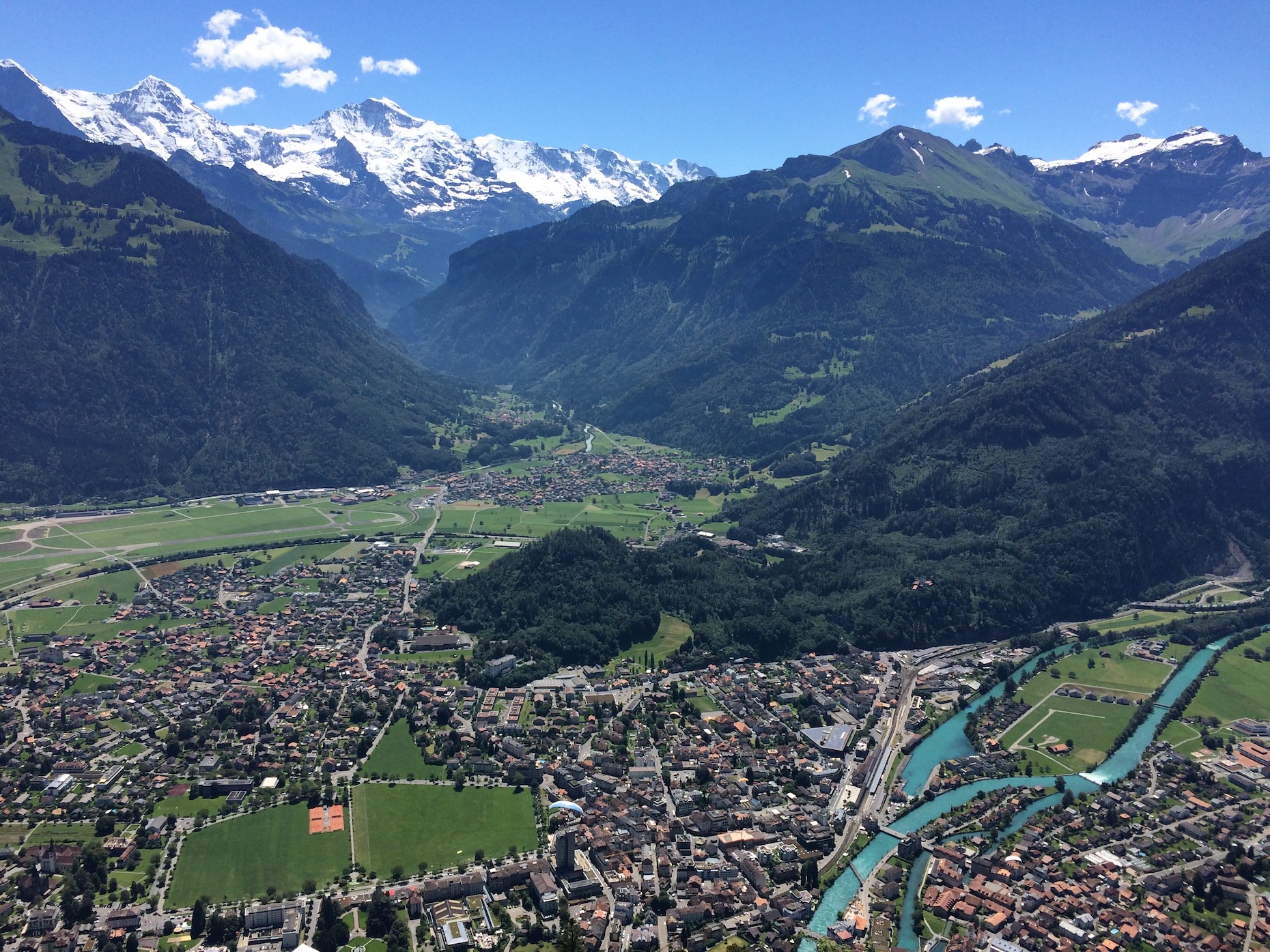
swiss alps (center)
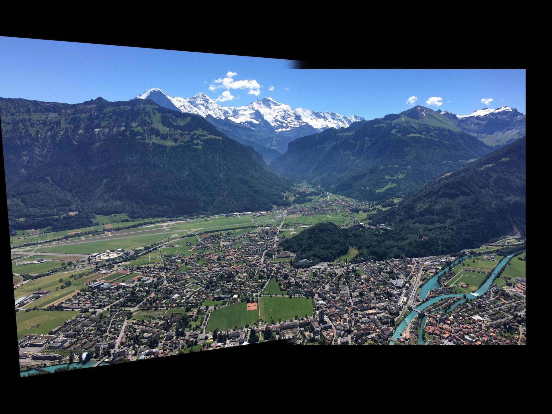
swiss alps mosaic
across the charles river
across the charles river mosaic: extra cropped (this photo set was very misaligned)
across the charles river (left)
across the charles river (center)
across the charles river (right)
across the charles river mosaic: cropped
// part b: feature matching and autostitching //
Harris Corner Detection
First, we find some potential interest points by using the harris.py interest point detector--with a small modification to use corner_peaks instead of peak_local_max to further filter out corner-like interest points. For each coordinate $(x, y)$, the Harris detector uses a sliding window of neighboring points to see how much the intensity $h$ changes when the window is moved in all directions; corner-like points will have large changes in intensity in every direction. These corner-like points are the interest points the detector will favor and find for us.
new york city skyline
NYC skyline (left)
NYC skyline (center)
NYC skyline (right)
overlooking prague
prague (left)
prague (center)
surrounded by the swiss alps
swiss alps (left)
swiss alps (center)
across the charles river
across the charles river (left)
across the charles river (center)
across the charles river (right)
Adaptive Non-Maximal Suppresion
Next, we use Adaptive Non-Maximal Suppression, or ANMS, to narrow down our interest points even further by making sure the selected points are evenly distributed across the image. Points that are too close together won't give us a very good homography transformation; and, in addition to giving us a more evenly spaced coordinate distribution, throwing out points that are too close together will also speed up our algorithm.
For each coordinate $(x_i, y_i)$, we calculate the radius at which $(x_i, y_i)$ is a local maximum with its peak intensity $h_i$ to all other points $(x_j, y_j)$: $r_i = min_j |(x_i, y_i) - (x_j, y_j)|$, s.t. $h_i < c_{robust} * h_j$. After finding each coordinate's local maximum radius, we take the first $z$ coordinates with the largest radii, where $z$ is a the number of points needed to be kept. Here, we've set $z = 300$.
new york city skyline
NYC skyline (left)
NYC skyline (center)

NYC skyline (right)
overlooking prague
prague (left)
prague (center)
surrounded by the swiss alps
swiss alps (left)
swiss alps (center)
across the charles river
across the charles river (left)
across the charles river (center)

across the charles river (right)
Feature Descriptors and Feature Matching
After filtering out enough interest points, we create feature descriptors that roughly describe each Harris point and its surrounding neighborhood. For each interest point, we select a 40x40 patch surrounding the coordinate. We then convolve the patch with a Gaussian filter and subsample it down to an 8x8 patch. Doing so creates a patterned patch that preserves only low frequencies, which acts as a rough guide to what the corner looks like.
Because different images may have different intensity values but still have the same general pattern, we want to adjust for bias/gain by subtracting the mean from each pixel in the patch and then dividing by the standard deviation. This will normalize the patches.
Once we've collected the feature descriptors for each interest point of both images, we look for matching descriptors in the other image. We only keep the interest points with matching feature descriptors, and pair them up as corresponding points. There is a certain error percentage in which we still treat the feature descriptors as matching in order to account for minor noise; here, we've set it to either 0.2 or 0.3.
feature descriptors
RANdom SAmple Consensus
Finally, we run the RANSAC algorithm on our selected interest points to find the best four corresponding coordinates to transform our image with.
1. Select four random corresponding coordinates from the matched up interest points.
2. Compute the homography matrix $H$ with these four points.
3. For every other point $(x, y)$ and corresponding point $(x', y')$ in our interest points, compute $(x'', y'') = H * (x, y)$. Count the number of $(x'', y'')$ that are very close to $(x', y')$, its actual corresponding point. In other words, how good is the current homography $H$ at mapping as many corresponding corners to where they should be?
4. Repeat 1-3 for many iterations.
5. Choose the best transformation matrix $H'$ that mapped the most correct corners to where they should be.
6. Use $H'$ to warp the image. Blend the warped images into a mosaic at their overlapping seam.
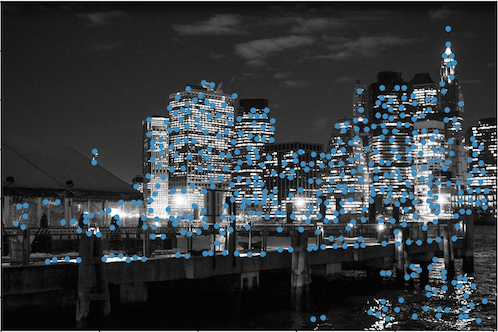
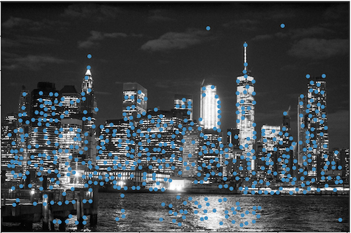
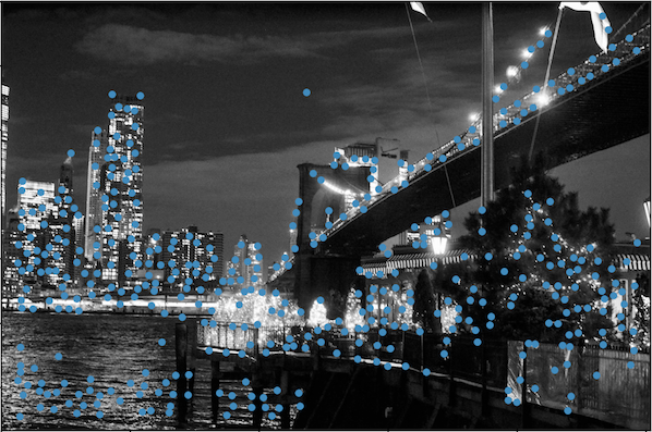
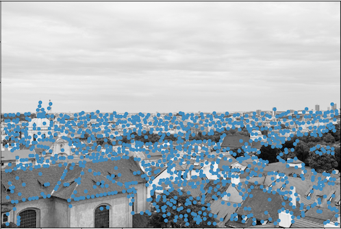
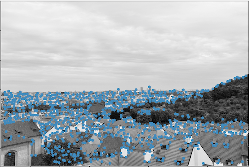
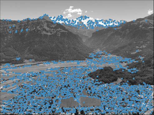
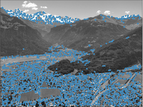
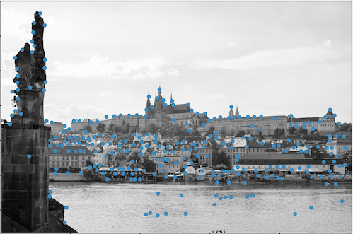
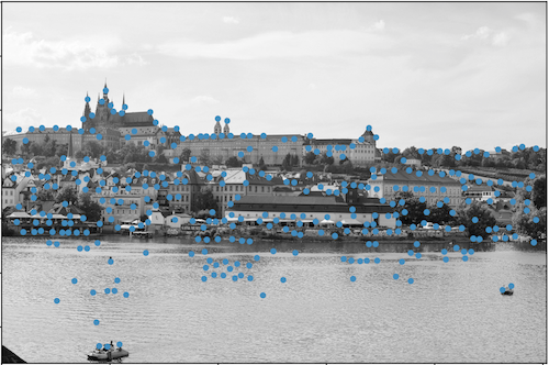
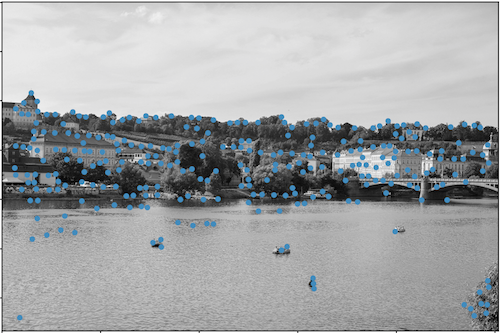
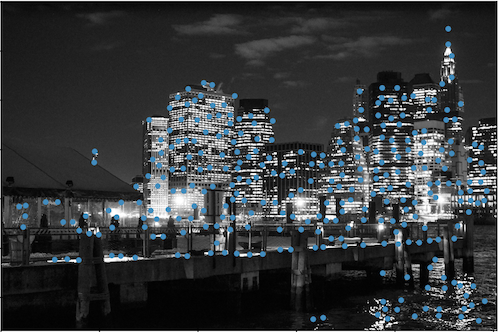
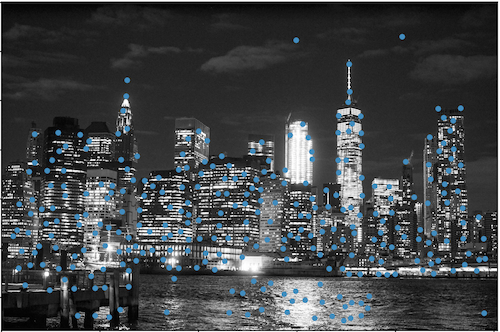
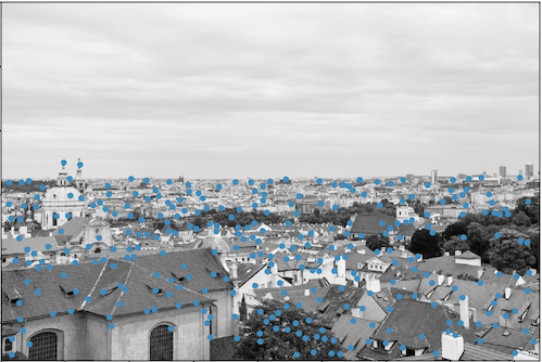
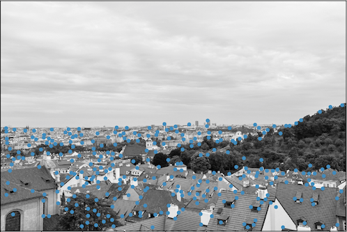
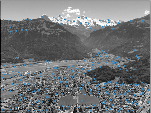
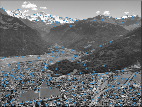
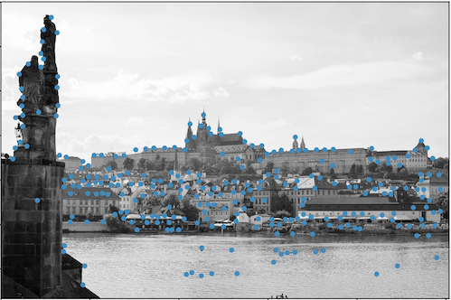
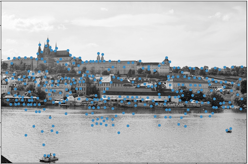
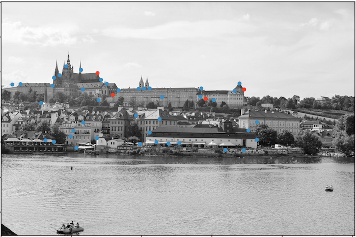
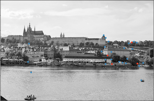
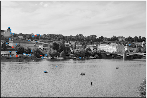
In the images below, the blue dots are the coordinates that have been found and filtered by the Harris detector, ANMS, and feature descriptor matching. The four red points are the four chosen coordinates for the final homography transformation.
new york city skyline
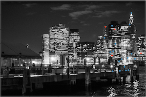
NYC skyline (left-center)
NYC skyline (left-center)
NYC skyline (right-center)
NYC skyline (right-center)
overlooking prague
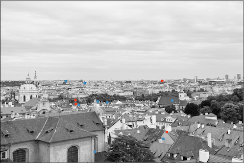
prague (left)
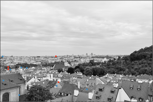
prague (center)
surrounded by the swiss alps
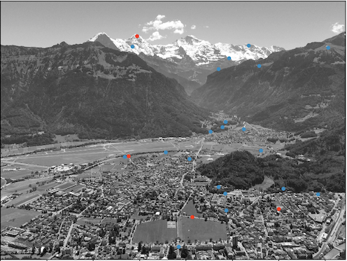
swiss alps (left)
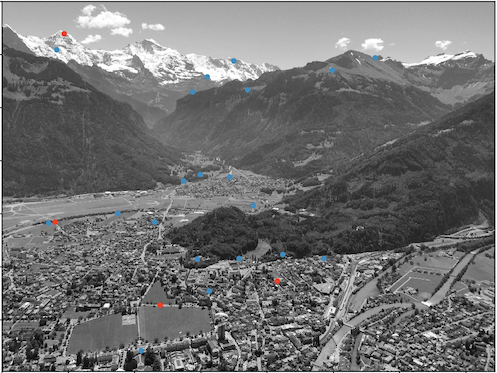
swiss alps (center)
across the charles river
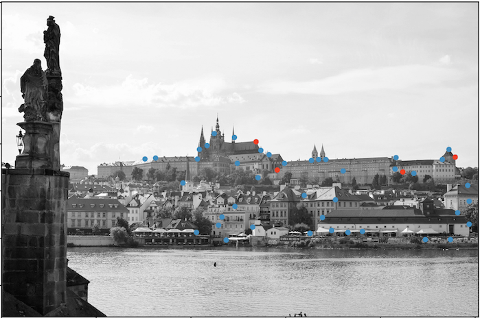
charles river (left-center)
charles river (left-center)
charles river (right-center)
charles river (right-center)
Mosiac Blending
new york city skyline
NYC skyline (left)
NYC skyline (center)
NYC skyline (right)
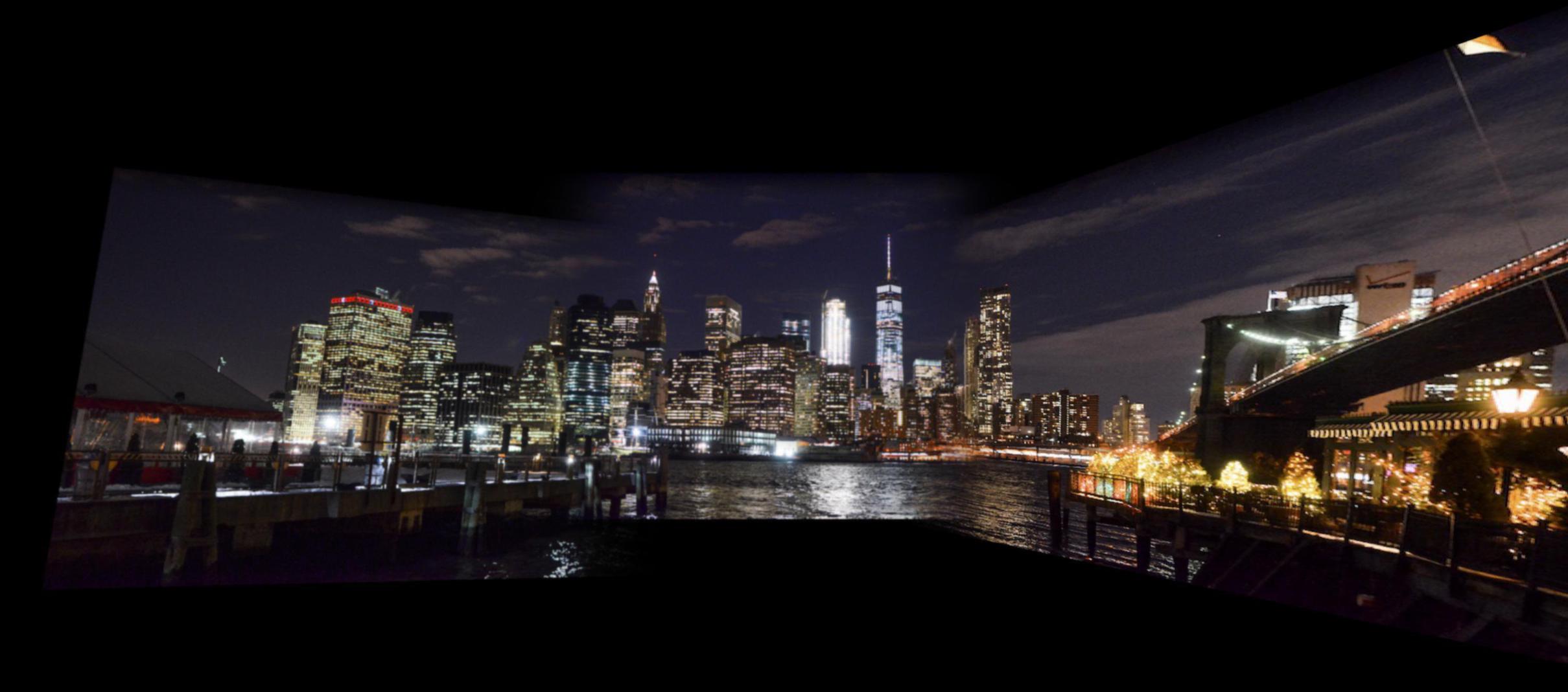
Automated stitching: NYC skyline mosaic
Manual stitching: NYC skyline mosaic
Winner: manual stitching. I believe it is because the images don't have high enough contrast for automated detection and matching since it's a night image. It was hard to align the center and right images correctly with autostitching. We can see that the shoreline by the bridge is not lined up very well.
overlooking prague
prague (left)
prague (center)
automatic stitching: prague mosaic
manual stitching: prague mosaic
Winner: both! Although we can see that the two mosaics aren't exactly the same, they're both pretty much spot on.
surrounded by the swiss alps
swiss alps (left)
swiss alps (center)
automatic stitching: swiss alps mosaic
manual stitching: swiss alps mosaic
Winner: both! Although we can see that the two mosaics aren't exactly the same, they're both pretty much spot on.
across the charles river
across the charles river (left)
across the charles river (center)
across the charles river (right)
automatic stitching: across the charles river mosaic
manual stitching: across the charles river mosaic
Winner: automatic stitching. In the manual stiching, the right image seems to be warped in the wrong direction, and we can see that the shoreline in the right image isn't straight, but going away from us. The automatic stitching gives a straighter shoreline, which more closely resembles what the river looked like if we were looking out at the other shore.
Conclusion
It was really cool to see how well RANSAC works, after learning about how simple it was to implement in class. Even though the points are selected at "random", the algorithm often provides us with really good corresponding points for us to use in our homographies, which is amazing!