Part A
Overview
For this project, we utilize projective warping to composite multiple images from different perspectives into image mosaics.
Part 1 - Recovering Homographies
In the first part we get the parameters of the transformation matrix between the images we sampled. The transformation matrix is the homography matrix p’=Hp, where H is a 3x3 matrix. There are actually on 8 degrees of freedom, so h33 is actually just set to 1. We compute H by first solving the below matrix equation. We use least squares since using simple inverse matrix multiplication would fail if we had more than 4 sample points. After getting the values of the h vector, we reshaped it to the square 3x3 matrix.

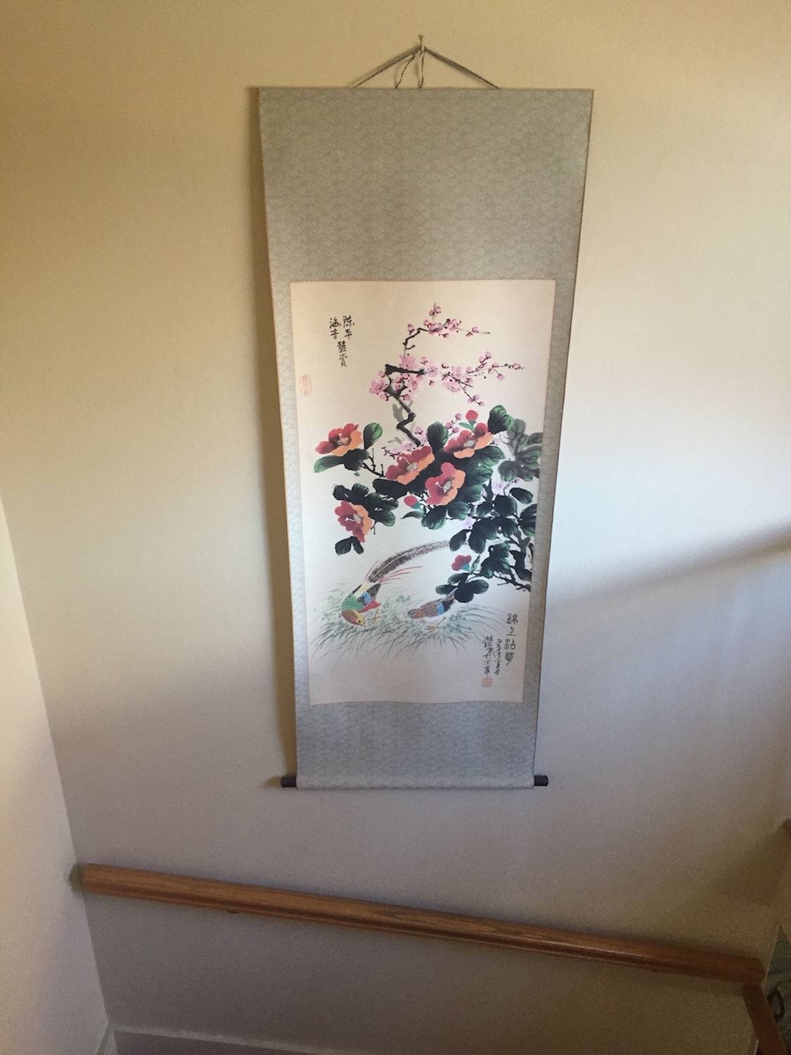
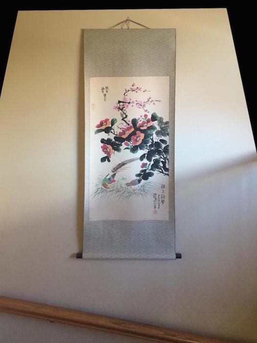
Part 2 - Image Rectification
After retrieving the homography, we do some test warps and warp some images so that it appears that we have a frontal perspective of it. To do so, we use forward warping with the homography matrix on the pixels of the original image to the correct position in the new image.
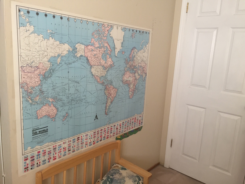 Before
|
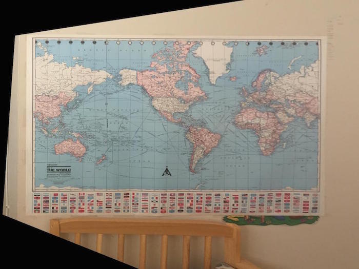 After
After
|
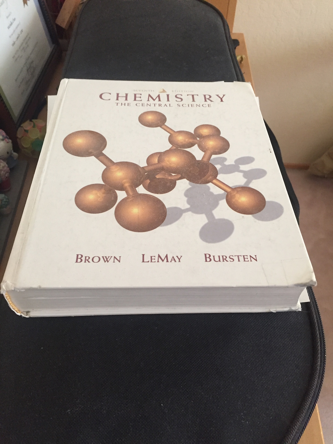 Before
|
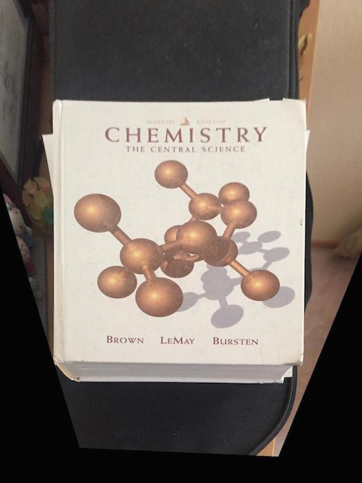 After
After
|
 Before
|
 After
After
|
Part 3 - Image Mosaic
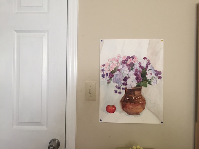
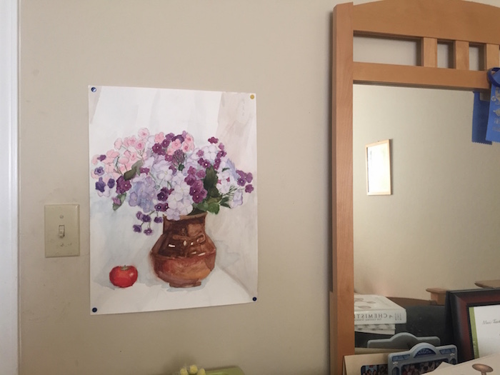
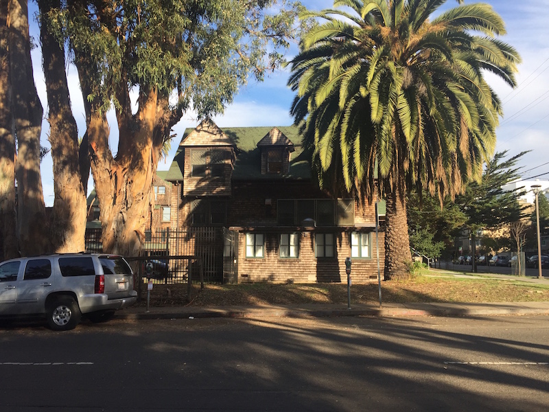
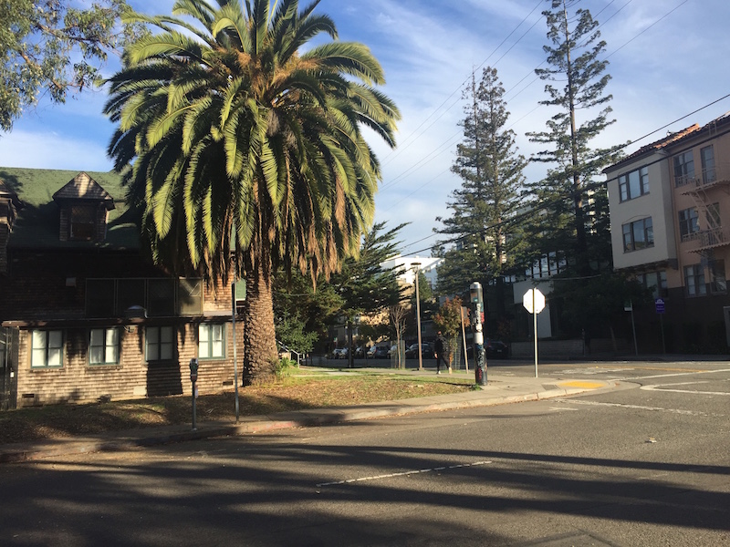
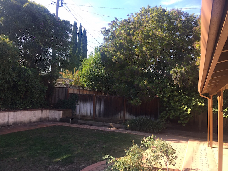
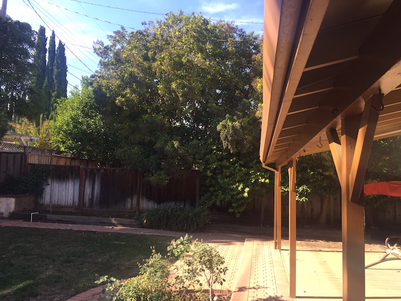
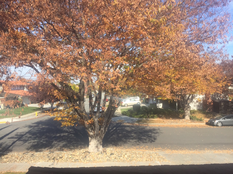
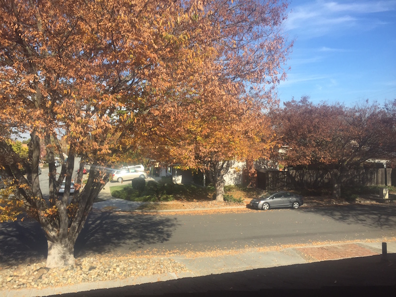
To create the image mosaic, I took two pictures of the same image in different perspectives with some overlap. Then I warped one of the images into the perspective of the other image using the previous steps, and blended them together using linear blending with a gradient mask. Because some of the data from the images get lost after warping, I padded both images to be twice the original size before doing the warp and blending. The images are a little blurry and have some artifacts, but I believe that it was mostly because I moved my hands between images or subjects in the image moved a bit.
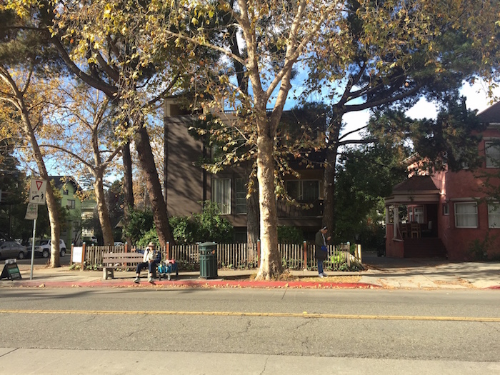 Source image 1
|
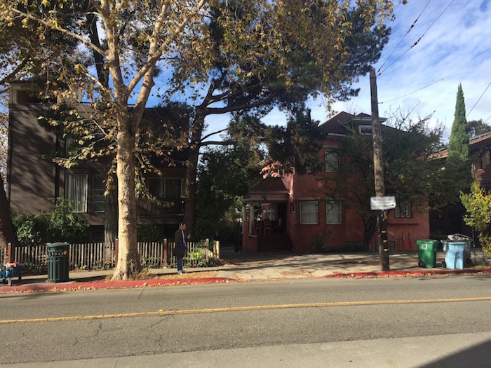 Source image 2
|
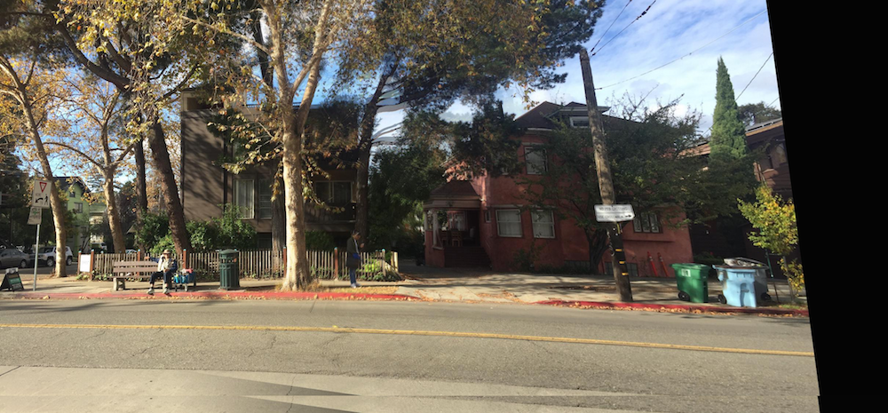 Image mosaic
|
 Source image 1
|
 Source image 2
|
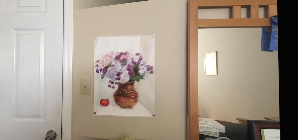 Image mosaic
|
 Source image 1
|
 Source image 2
|
 Image mosaic
|
Part B
Overview
Continuing off of part A, we want to be able to automate the image mosaicing process by using a simplified version of the algorithm presented in the paper "Multi-Image Matching using Multi-Scale Oriented Patches" by Brown et al.
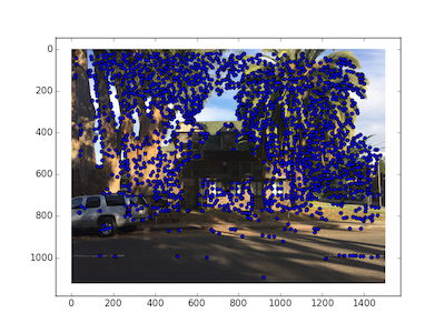
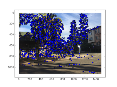
Part 1 - Harris Interest Point Detector
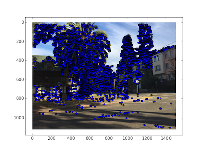
We first determine points of interest in the image by using a Harris corner detector, the code of which was provided to us. The idea is to look at 3x3 windows of pixels, and find the pixel with the a local maximum value to the corner strength function.
Harris points on sample image
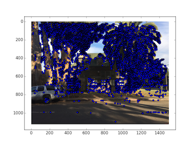 Harris corners on Source Image 1
|
 Harris corners on Source Image 1
|
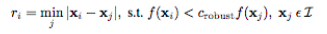
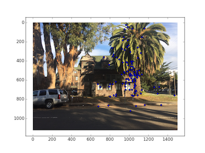
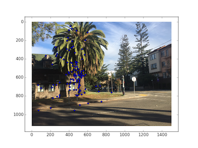
Part 2 - Adaptive Non-Maximal Suppression
Currently our images have a lot of Harris corner points, so we try to narrow down the subset by applying Adaptive Non-Maximal Suppression on the set of points. ANMS is useful because it will narrow down the set of points such that they are spatially well-distributed. In ANMS, for every point in the set, we calculate the distance to the closest point whose corner strength value multiplied by some robustness value is greater than the examined point's robustness value. The minimum suppression radius is given by the equation below. After we have gathered the r-value for every point, we pick the top n points with the maximum r-value. In my case, I just picked the top 20% of points.
Harris points after ANMS
|
Before ANMS on Source Image 1
|
 After ANMS on Source Image 1
|
|
Before ANMS on Source Image 2
|
 After ANMS on Source Image 2
|
Part 3 - Feature Descriptor extraction and Feature Matching
Finally, we want to keep only the interest points that match between the two images. First, we want to generate a feature descriptor vector for every set of points. We do this by generating a 8x8 descriptor patch, which is averaged from a larger 40x40 patch centered around the point, with a spacing of 5 pixels. We generate a higher-level descriptor to avoid aliaxing. We transform this 8x8 patch into a length 64 vector. In feature matching, for every point in source 1 we find the best match and the second-best match pixels from source 2. We'll call the SSD value generated from these points NN1 and NN2. The idea is that if it is a correct match, then the second-best match pixel must have an SSD value that is much larger than the best-match. To do that, we kept pairs where NN1/NN2 < 0.4.
Interest Points from Feature Matching
|
Harris corner points on Source Image 1
|
After ANMS on Source Image 1
|
 Matching interest points on Source Image 1
|
|
Harris corner points on Source Image 2
|
After ANMS on Source Image 2
|
 Matching interest points on Source Image 2
|
Side by Side comparison of Matching points
|
Final Interest points on Source Image 1
|
Final Interest points on Source Image 2
|
Part 4 - Computing the Homography matrix using RANSAC
We use RANSAC as a more robust way of calculating the homography matrix. First, we select 4 random points to compute the homography matrix. Then, for every point in one image, we warp the point with the calculated homography matrix, and if the point is less than some threshold distance away from the true coordinates (we set this threshold to 10), then we count this point as an inlier. We keep the largest set of inliers we've seen so far and repeat the above process many times. After many trials, we return a homography matrix calculated from the largest set of inliers we've seen.
Final Images
 Source image 1
|
 Source image 2
|
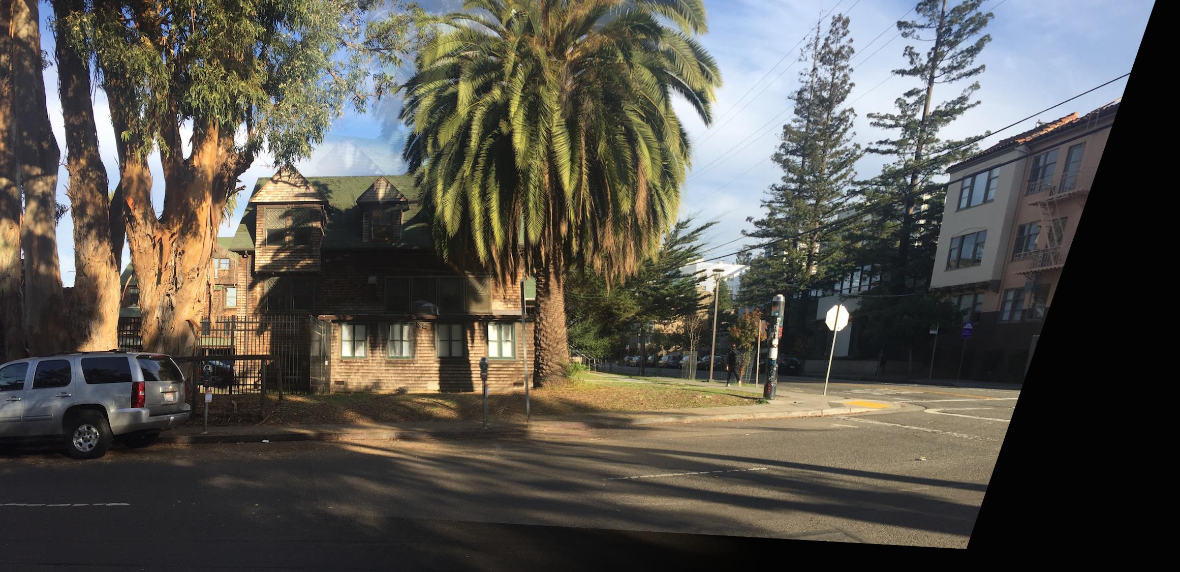 Image mosaic
|
 Source image 1
|
 Source image 2
|
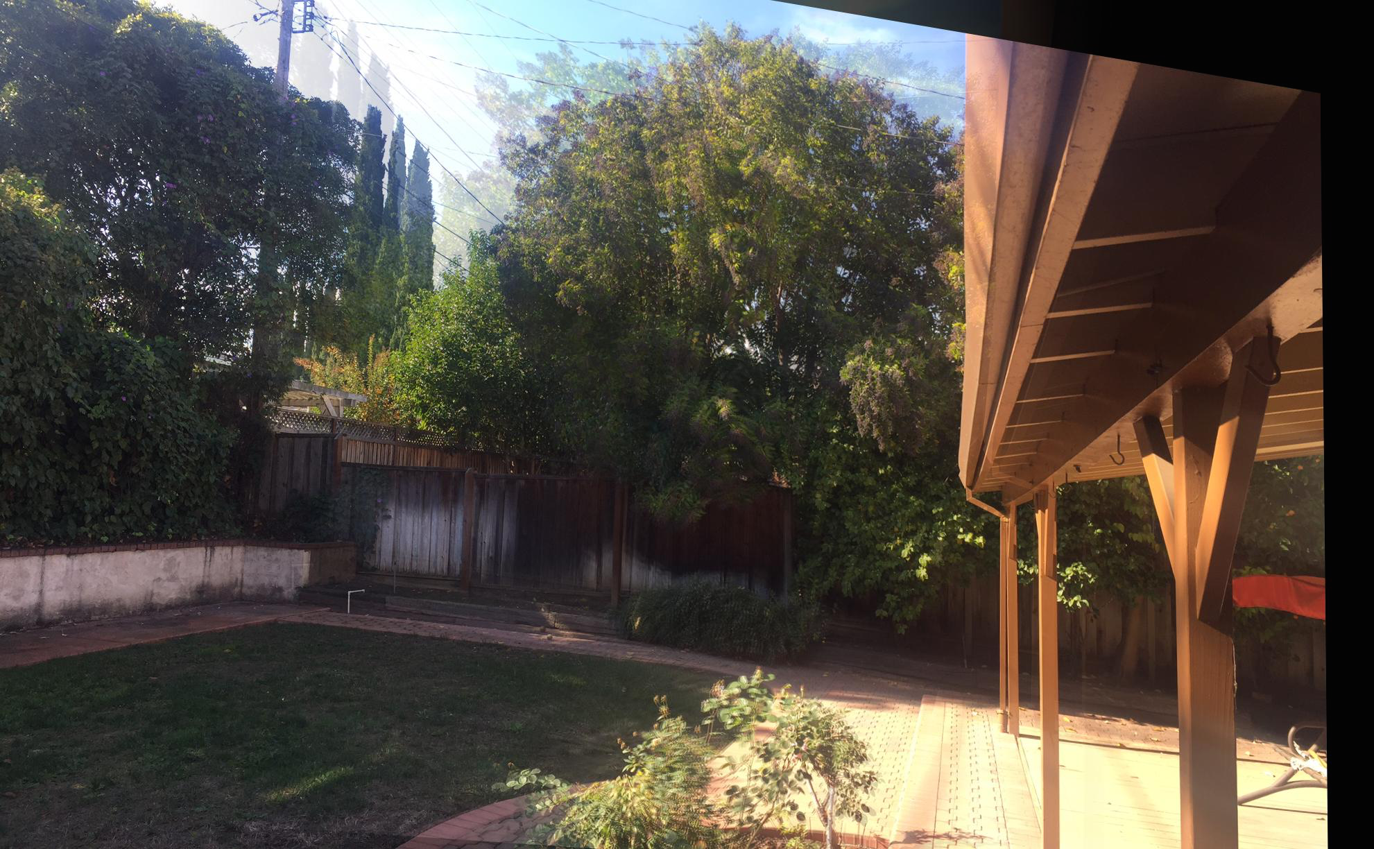 Image mosaic
|
 Source image 1
|
 Source image 2
|
 Image mosaic
|
Summary
This was a very difficult process to do, mostly because taking good photos that would align well without fancy equipment was quite difficult. The above images don't seem to align very well, but is mostly attributed to using images that were not taken properly/aligned on the same plane. But overall, it was pretty cool to see the points generated and to see the algorithm pick out the matching points.