Part A: Image Warping and Mosaicing
Overview
This project warps images with projective transforms using the homography between point correspondences and blends the warped images into a mosaic.
Recover Homographies
I first captured images with overlapping fields of view by changing the direction of the camera and select 4 point correspondences from the images. Given points p=(x, y) and p'=(x', y'), the homography is: p' = Hp (see left image from lecture below). To solve for H, write as system of equations:
x' = x*h1 + y*h2 + h3 - x'*x*h7 - x'*y*h8
y' = x*h4 + y*h5 + h6 - y'*x*h7 - y'*y*h8
and construct matrices A as a (2n, 8) matrix of coefficients and b as a (8,) vector of points (see right image below). Since Ah = b, solving for h through least squares give us 8 values of H (the homography matrix). Finally, add h9=1 and then reshape H into a 3x3 matrix.
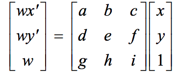
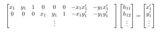

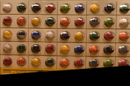
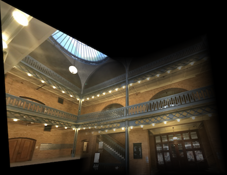
Image Rectification
Using H, we can warp the images such that the planes are frontal-parallel with four points in the source image warped into a square.
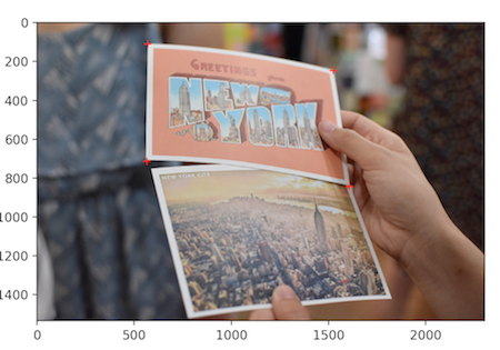
Original image with 4 selected points
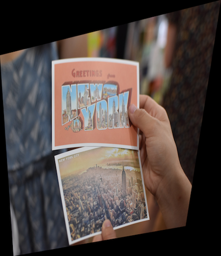
Warped image
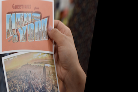
Rectified (cropped)
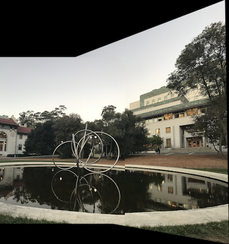
Mosaics
For this part, the idea is to center an image and warp the other image(s) to the centered image. I first pipe the corners of an image through H to get the warped image boundaries, then create a new array with size equal to the total mosaic shape, and fill this array with the blended warped image and centered image.
For blending, I used alpha masks for the images to blend areas of overlap by taking a sum of the images weighted by their respective alpha masks before putting this result in the final image array.
Results
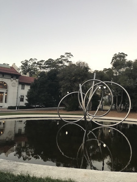
Image 1
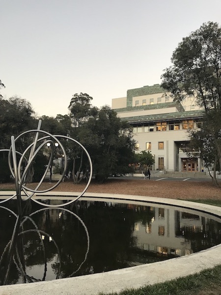
Image 2
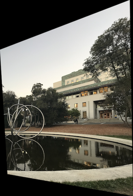
Warped image 2
Stitched without blending

After blending
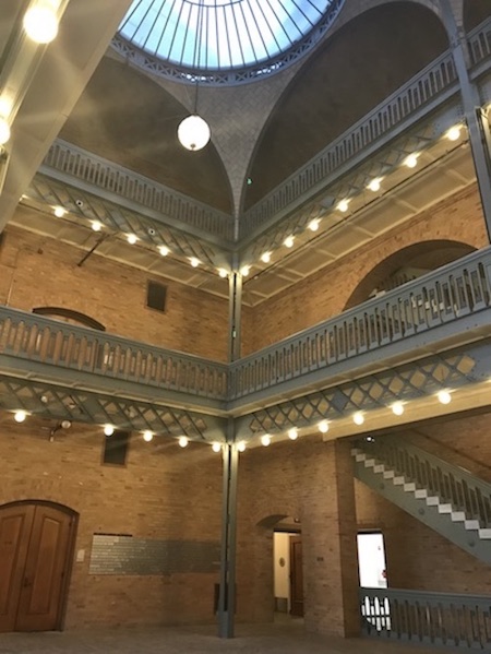
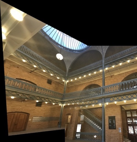
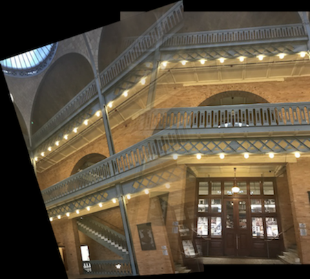
Image 1
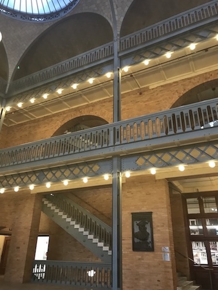
Center image 2
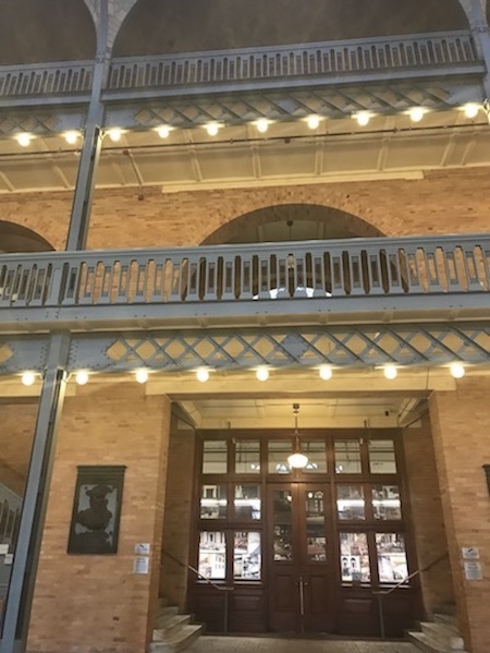
Image 3

Images 1 and 2
All 3 images
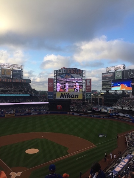
Image 1
Warped image 1
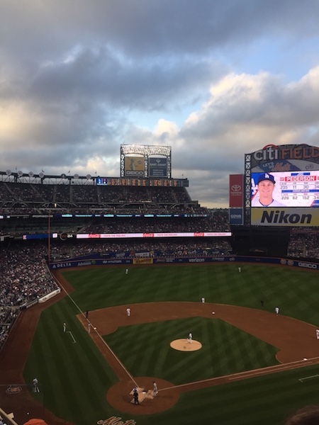
Image2
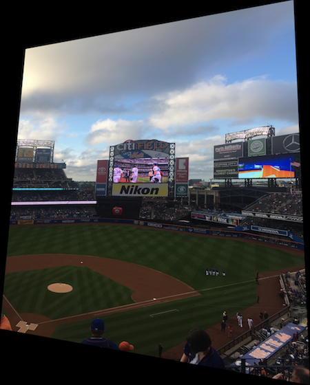
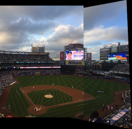
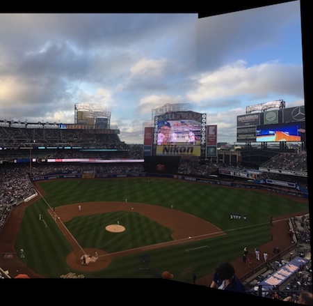
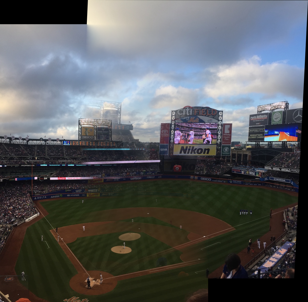
The left image below is without blending and right is with linear blending. This one was a little messed up due to the fact that the images, when taken at the time, weren't intended to be projective so the scoreboard is misaligned though the baseball field lines blended more seamlessly.

Takeaways
From this project, I learned about homography and image rectification, and how to combine previous blending techniques to create cool mosaics.
Part B: Feature Matching for Autostitching
Overview
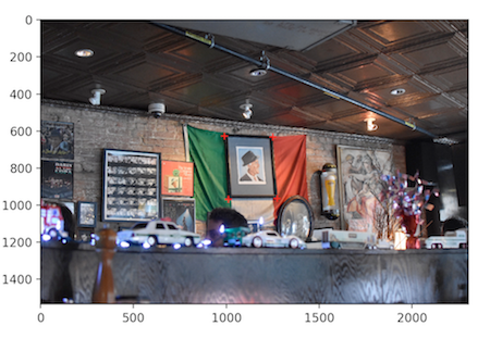
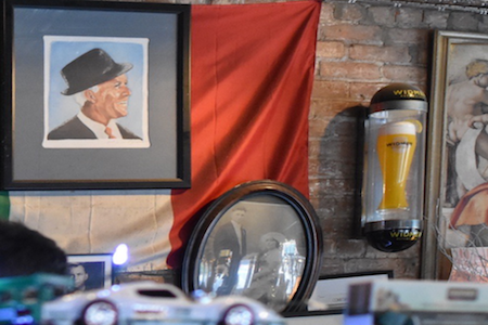
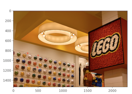
The main task here is to automate the process of selecting points and stitching images to create panoramas. The original images I use are:
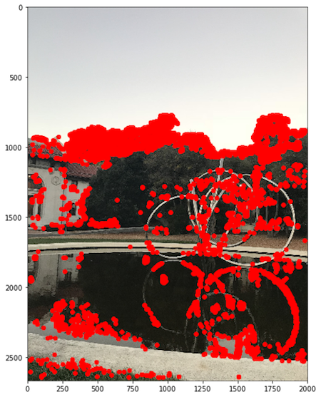
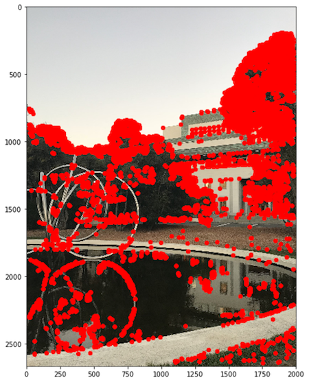
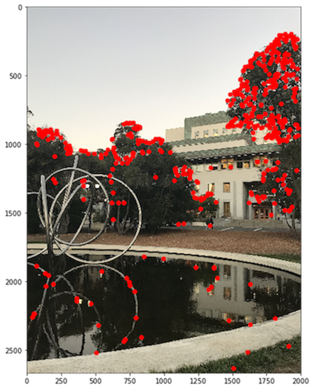
Detecting corner features in an image
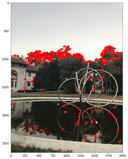
With adaptive non-maximal suppression, the approach is to define a minimum suppression radius r, and keep only points with a maximum corner strength in their neighborhood of size r. Following the paper by Brown et al., I defined r to be the minimum distance between point1 and point2 where the corner strength f of point1 < 0.9*f(point2). The end result is 500 points that are better distributed spatially across the image.
Feature Descriptor Extraction
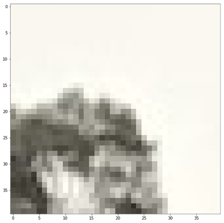
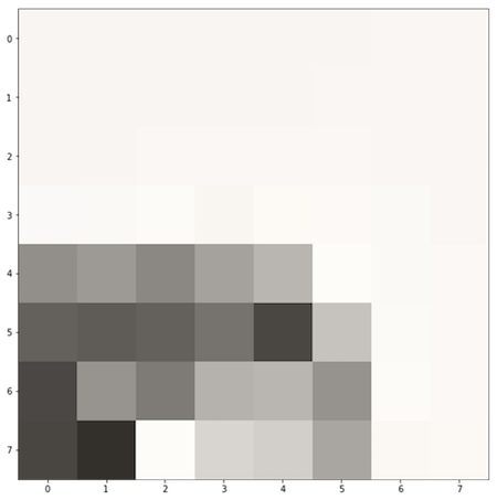
To extract a feature that corresponds to each point, I take a 40x40 patch around each point and sample by applying a Gaussian filter to make the patches less sensitive to the exact feature location. Then, I sample every 5th row and column to get a 8x8 patch that is bias/gain-normalized.
Below is a 40x40 patch (left) downsampled to an 8x8 patch (right):
Feature Matching
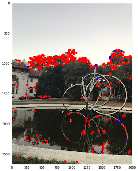
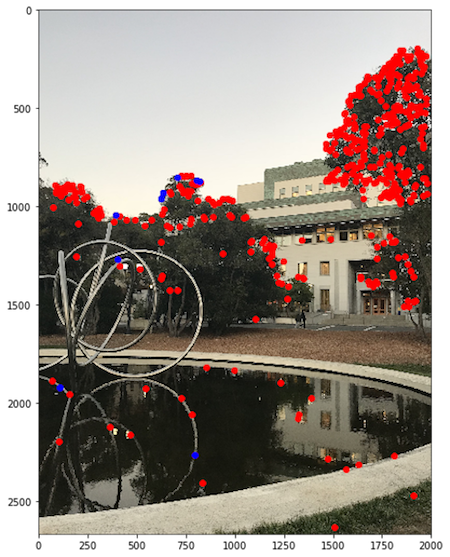
To match feature points, I use dist2 to find the most similar pair of 8x8 descriptors. The implementation is to calculate SSD of image1's feature descriptors with image 2's, and for each row, find the nearest neighbor (1-NN) then the second nearest neighbor (2-NN). The feature matching function returns the indices as (i, j) pairs where the ratio of 1-NN to 2-NN < 0.6. The results below show the points with feature matches in blue and discarded feature points in red.
Homography with RANSAC
With Random Sample Consensus (RANSAC), I randomly select four pairs of points, compute homography matrix H and find SSD(p', Hp) where p' is the points of image2, and p is the points of image1. I then determine inliers as points within some defined threshold e=1000. I repeat this process for 1,000 iterations to find the best homoegraph (with largest set of inliers) to warp the image with functions from part A. Thus the RANSAC function returns the homography matrix H that gives the largest set of inliers.
Resulting Mosaic
After RANSAC, the process of warping and stitching the two images follow the procedure from part A. The auto-stitched results are shown alongside those from Part A, though I had a hard time finding threshold values yielding perfect stitches since RANSAC is problem-specific. Unfortunately, there is misalignment of coordinate points resulting in imperfect mosaics.
Results
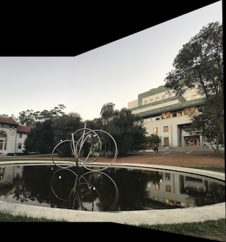
Manually stitched
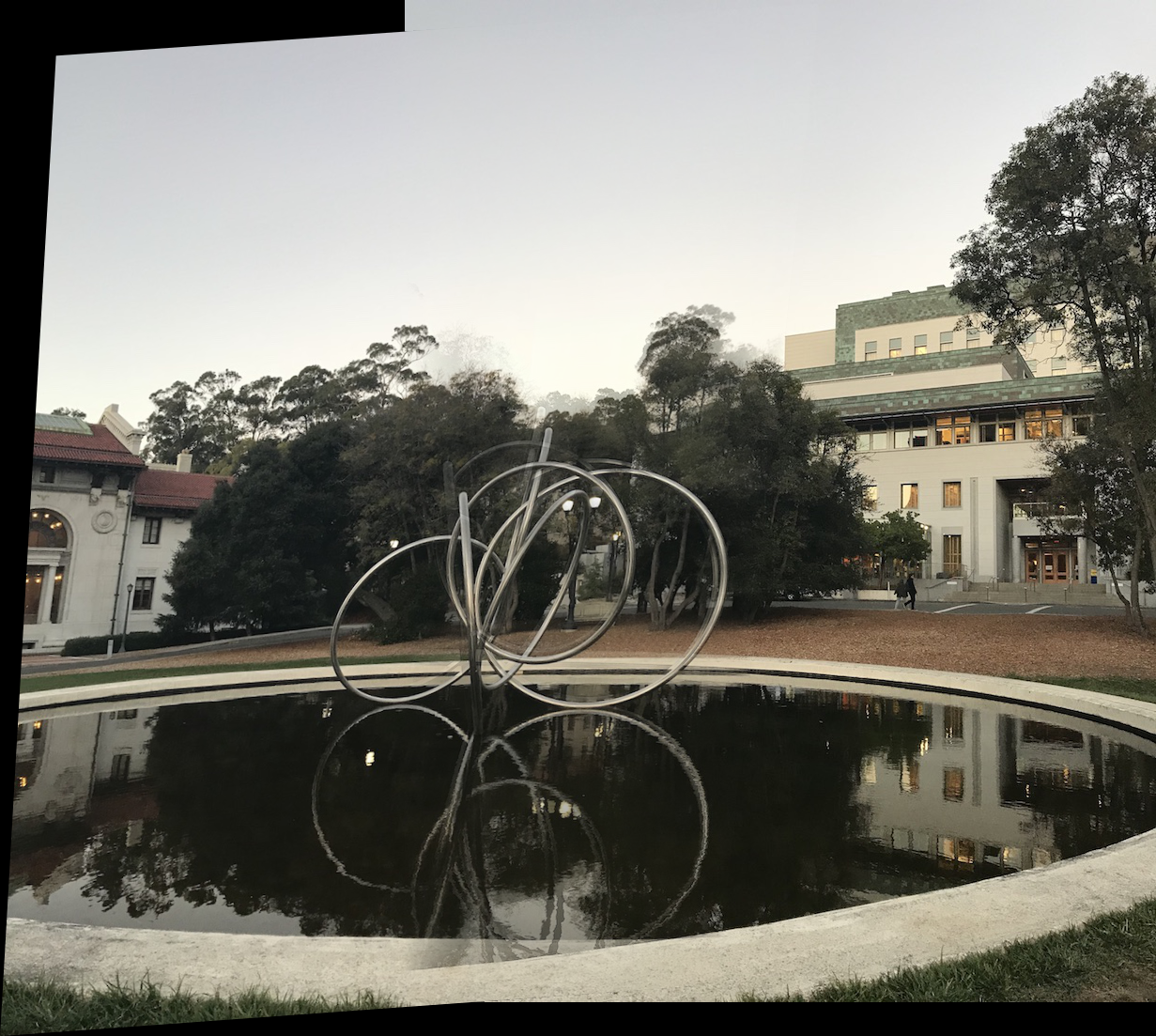
Automatically stitched
Manually stitched
Automatically stitched
Manually stitched
Automatically stitched
Takeaways
It was neat to automate the entire process of selecting coordinates between the input images, and combining past concepts and techniques such as Gaussian fliters. Though some challenges included understanding the paper and finding the right threshold values for RANSAC, I learned alot from the process of implementing these algorithms.