CS 194-26 Project 6
Image Warping and Mosaicing - Part 1
Completed by Alex Krentsel
Yosemite stiched together and blended with optimized feathered blending
Description
In this project, we are going to be stitching images together to create image mosaics. We first get a pair of images take from the same point in space, only turning the camera to take the second image, with part of the image overlapping. We then define at least 4 corresponding points between the two images. We use this information to solve for a homography matrix, then apply this matrix to transform the first image into the "plane" of the second image, and translate the images to line up correctly, producing a panoramic mosaic image. We can optionally use some blending methods to make the alignment look smoother, as I have done below.
Shooting the Photos
I shot a a bunch of sets of photos for this project. I also dug into my Google Photos and pulled out some old photos of mine from Europe to use. I also experimented with some photos from online of Yosemite and other places.
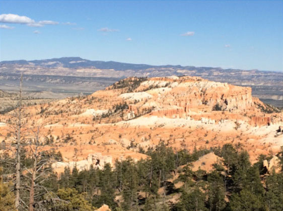
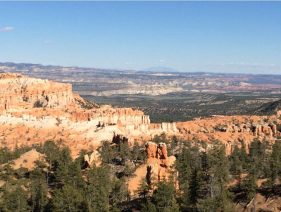
Here are a few of the images that I gathered:
I then labeled the pairs of images that I collected with sets of 4 corresponding points and stored them in a text file for each pair of images.
Recovering Homographies
Once I labeled the pairs of images with sets of corresponding points, I could proceed to find the matrix to trasnform the points in one image to the corresponding points in the other image. This matrix is called a
homogrpahy matrix. To find this matrix, we can set up a system of equations, where each equation comes from application of the homography matrix (which is made up of 9 unknowns):
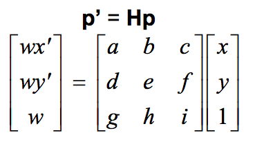
We can set
i to be 1, and therefore are left with 8 unknowns. Therefore we need 4 points to have a solvable set of equations, since each pair of points provides both an x and a y correspondance. We use linear least squares to solve for the 8 unknonws that we need to define our homography matrix. We use the homography equation in the future parts.
Image Rectification
Once we have a homograpy matrix, we can now change image perspective and apply rectification. In rectification, we select points in the image that correspond to a known shape in the real world and transform the image to match that known shape. See my results below:
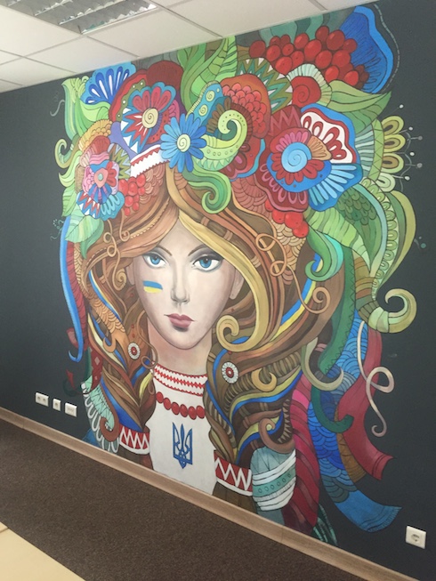
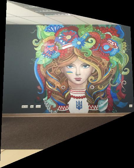
On the left is the original image, on the right we used a homagraphy to rectify the Ukrainian woman.
Mosaic Image Blending
Finally, once we have homographies working correctly, we can project images onto the same "plane" by apply the homographic transformation for the corresponding points between two images to the first image to map the first image to the "plane" of the second image. We then translate the first image by the amount dictated by the correspondance between the point mappings.
This can produce a result with a sharp edge between the two images, so we can use some feather-blending to smooth out the edge between the two images and make the mosaic loom more natural.
Results:
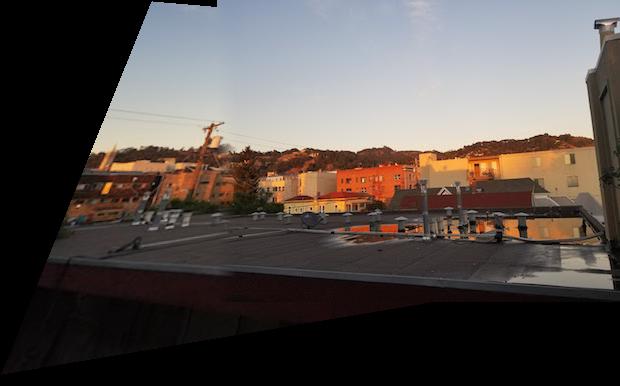
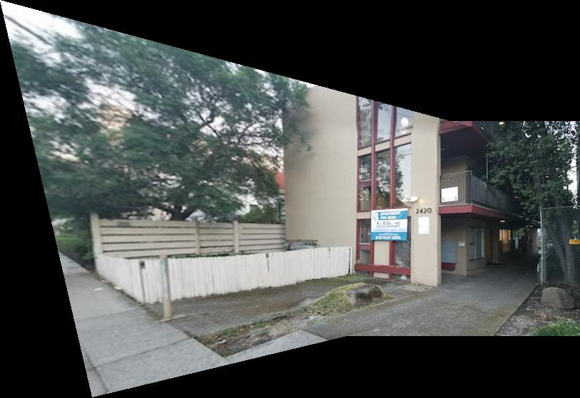
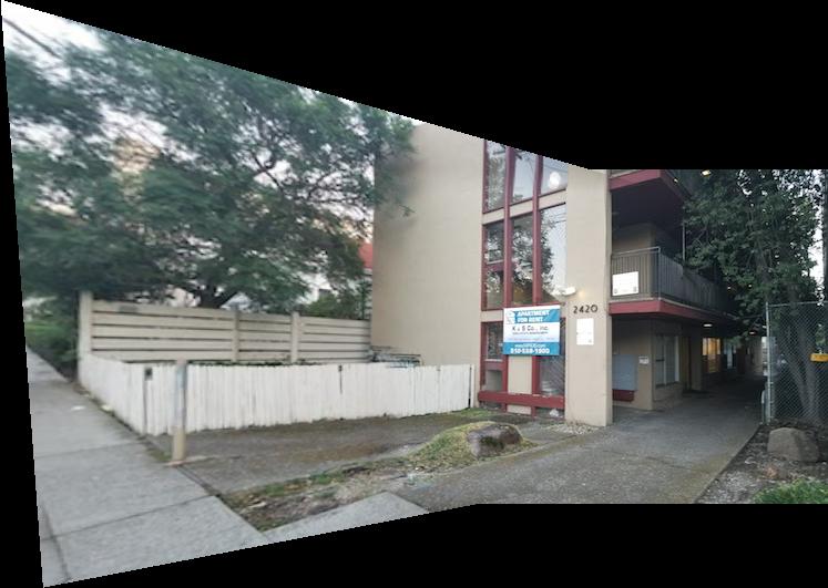
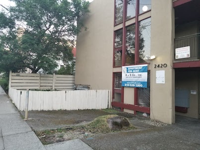
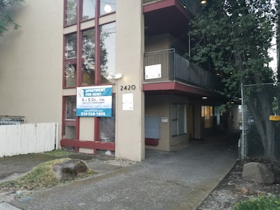
Apartment Photos
Combing these two images, I got these results:

Naive blending on the left, horizontal feathered blending on the right
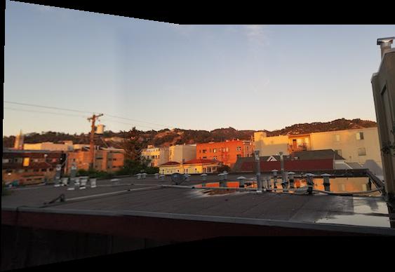
Now, this result looks pretty decent. But the horizontal feathered blending isn't perfect. Because the blending is only horizontal, you can still see the horizontal seams (in particular at the top). To deal with this, I made some modifications and added complementary vertical blending as well, producing this final result:
For the other two examples, I'll leave out the suboptimal blending result.
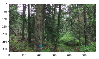
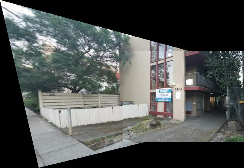
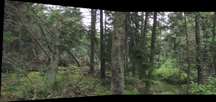
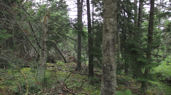
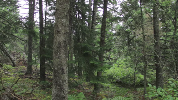
Forest Photos
Combing these two images, I got these results:
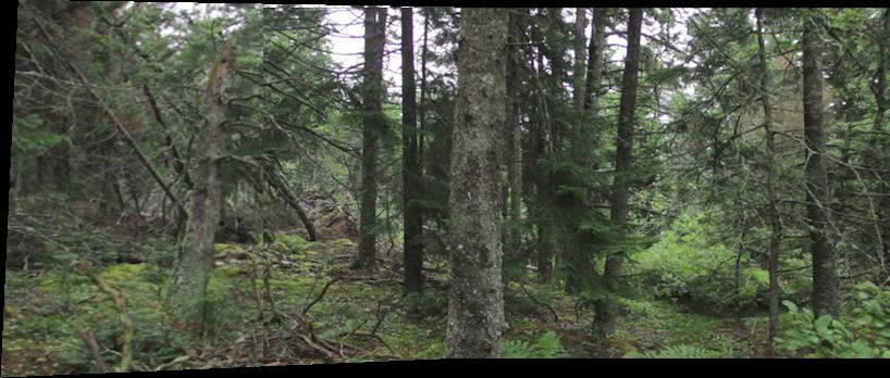
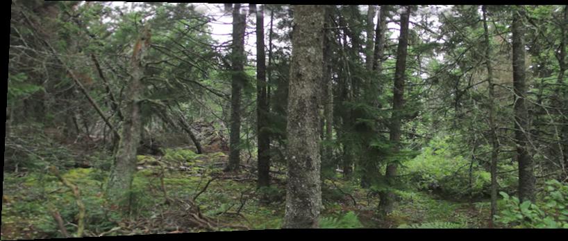
Naive blending on the left, optimized feathered blending on the right
This one turned out reasonably well as well, but there are some things that don't align exactly. I think this is because this is such a complicated image (lots of fine details), so it's easier to tell when something isn't perfectly aligned. Also, it was harder to match up points exactly because there weren't many hard corners, so some of the points could have been off by a little.
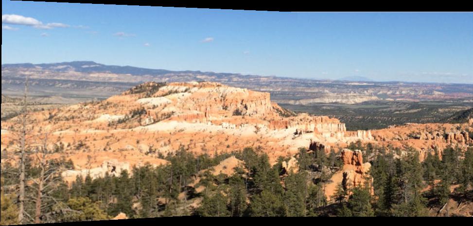
Yosemite Photos
Combing these two images, I got this result:
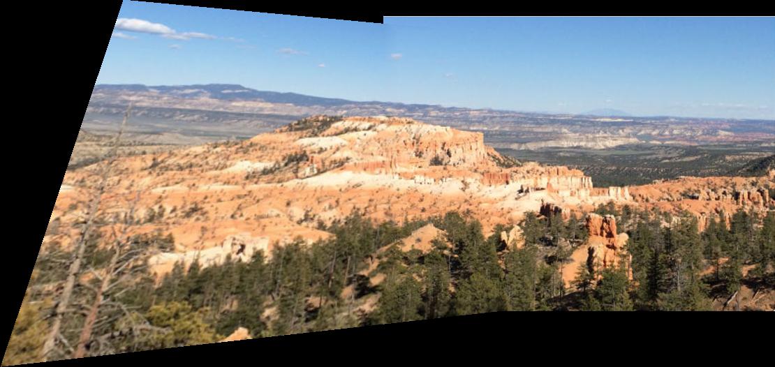
Optimized feathered blending
This one turned out really, really well. The seam is nearly impossible to see. The optimized blending makes it look great. I think it looks particularly good because the mountains are so far away, so any sort of accidental movement on the part of the camera is treated basically as error that is quite small and doesn't affect much.
Summary of What I've Learned
I've learned that homographies are super cool. It's especially amazing to see the additional power that we get by just adding one more corresponding point, as compared with the last project doing face morphing. An extra point of information let's us do way, way more things.
I've also learned that it takes a decent amount of thinking to figure out a nice way to blend the seam along two two slightly different images. Feathered blending isn't as easy as it seems. I'm looking forward to the second half of the project.
Feature Matching for Autostitching - Part 2
In this part of the project, we do the same thing as in part A, except that instead of soliciting points from the user for the homography calculation, we will find correspondance points automatically.
There are 6 steps for automatically computing the homographies automatically:
1. Detecting corner features in an image
2. Picking a subset of the corner features
3. Extracting a Feature Descriptor for each feature point
4. Matching these feature descriptors between two images
5. Use a robust method (RANSAC) to compute a homography
6. Transform the images using the homography matrix and stich them together
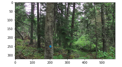
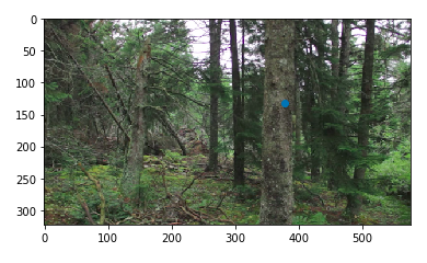
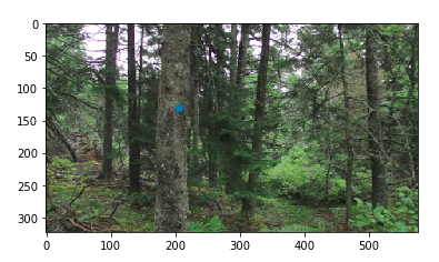
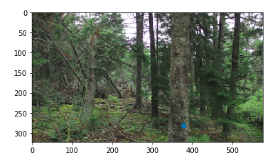
I will explain in more detail each of these steps below. I will walk through all of the steps with these two images:
For the other panoramas, I'll leave out the in between steps and only show the final results.
1. Detecting Corner Features
For detecting corner features, we use the harris interest point detector. To figure out how "cornery" a particular point is, we take a square, and wiggle it around that point, calculating the change in pixels as we wiggle it around. This, in effect, gives us a derivative for the change in pixel intensity due to movement. If a particular point is a vertical line, then horizontal motion will cause pixel intensity changes, but vertical movement won't at all. If it is horizontal, then the conclusions are swapped - except horizontal movement now doesn't change anything. If it is a corner, then movement in any direction resulting in a high pixel intensity change. We assign each point a "corneryness" score, and return all the points with a non-low corneryness score, along with their scores.
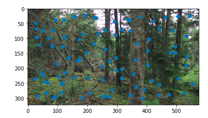
This gives the following result (with all the harris corners):
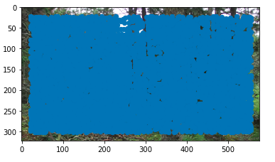
Notice that there is a crazy amount of them. In fact, there are so many, that the entire image just looks blue. This is likely because this is a forest, and so it is a very complicated image, and many pixels have high pixel intensity gradients, resulting in many pixels being above the cut off for "cornery-ness." This makes it even more impressive that our algorithm is able to find matching points in the end, as there are so many potential corners when we first start.
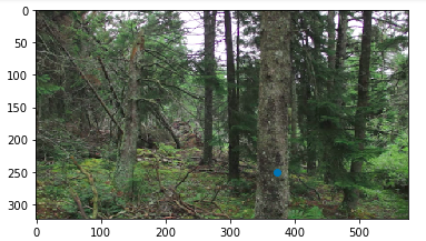
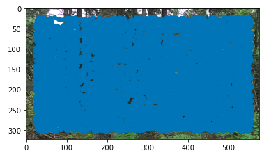
2. Picking a subset of points
As you can see above, this returns a lot of points. We want to take a subsample of these points to use for processing. Too many points will make the processing too slow and potentially run into more false matches later on. A naive solution would be to take points with maximally large corner scores and throw away the rest, but this may result in all of the points being located in a particular part of the image (not be spread out), and if that region happens to not be part of the overlap, then we wouldn't be able to find matches.
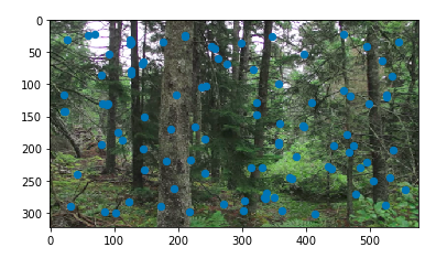
For the reason, we do ANMS. In ANMS, we minimize the following equation to get a list of suppression radiuses:

Intuitively, this says that for each interest point, we want to know the largest radius for which it is the most cornery. Then, we sort the interest points by their suppression radiusses and take the top n points. This gives us a result like this:
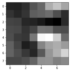
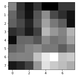
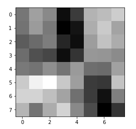
3. Extracting a feature descriptor
Now that we have a set of points, in order to compare them to each other and try to match them, we need to extract the images of the corners from the image in some way. For this, for each interest point, we take a 40x40 square around the interest point, and then downsample to an 8x8 patch. Note that for lower resolution images, we may need to start with something smaller than 40x40, so as not to include too much of the image. We also bias gain and normalize each of the patches, so that relative brightness differences don't affect our image matching.
Because our photos for the panorama were taken without any rotation, we don't need to worry about making these features rotation invariant. In a real setting, we would make them rotation invarient by also figuring out which direction the corners point in and rotating all extracted features to have the corners point in the same direction consistantly.
Here are a couple of extracted feature descriptors:
They look pretty bad, but this is to be expected, as we are down-sampling by a lot, and also normalizing and biasing, which make the corners much harder to recognize for us.
4. Matching Feature Descriptors
To match feature descriptors to each other, we take the list of feature descriptors for each of the images, and compute the pairwise distances between them. This works decently, but many mistakes are still made. To improve the performance, we use the Russian Granny Algorithm as discussed in class. We take the ratio between the first nearest neighbor and second nearest neighbor, and threshold that value, throwing away all pairs that are not past the threshold. The intuition here is that if a patch is close to both its first and second nearest neighbor, then it's not a very trustworthy match, so we just throw it away.
This gives us matching points in the two images:
5. RANSAC to Compute Homography
Now that we have a list of points that we think match, we need to compute a homography as before. However, we don't know which points are good matches and which ones aren't. We think that most are good, but we aren't guarenteed that all are good. To combat this, we use Random Sample Consensus (RANSAC for short). For a number of iterations, for every iteration we pick 4 points at random, compute the homography using those 4 points, then use that homography matrix to transform all of the interest points in one image to the other image and see how many are mapped correctly (inliers) and how many are mapped incorrectly (outliers). We use the homography matrix of the set of points that had the largest set of inliers. To get an even better homography matrix, we can recompute the matrix using all of the corresponding inliers (to help minimize error).
6. Compose the Images - Putting it all Together
Finally, we compose the two images together in the same fasion as in part A of the project. With these two forest images, we get the following result:
The result with provided correspondances on the left, the auto-corresponded result on the right
This is really good! It is especially impressive considering that we didn't provide anything other than the two input images. It is a magnitude better than the result with the same images from part 1.
Result Comparison
On the left is the result when manually providing correspondances, and on the right is the result of automatically finding correspondances:
This one looks much, much better. All of the lines line up correctly.
This one also looks very, very good. This is my favorite. You can't tell at all where the seam is.
This one looks better, but not as drastically better as with the other two examples. You can tell that it's a bit better because the light fixture in the building on the left isn't doubled as it is in the panorama from part 1.
It is completely crazy to me how the auto-created results are not only on par with my hand-matched mosaics, but actually an order of magnitude better. Yosemite, in particular, stands out. That image looks like it was taken by a single camera in a single photo. There is no point that I can tell that it was a composed photo. I think it worked particularly well because everything in the image was so far away from the camera.
My favorite part was playing around with more images that I'd taken and NOT having to provide manual correspondances. The amazing quality without providing correspondances made it really fun to play with. That was the coolest part that I learned - with a proper pipeline, you can accomplish pretty difficult tasks automatically and with very high quality.
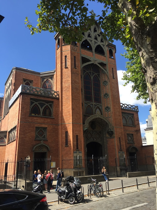
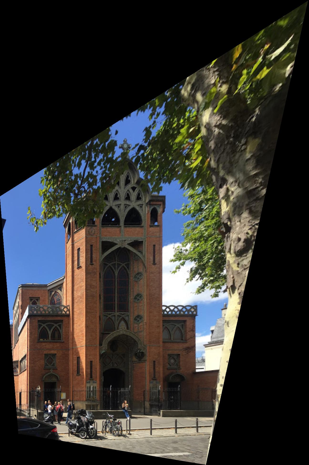
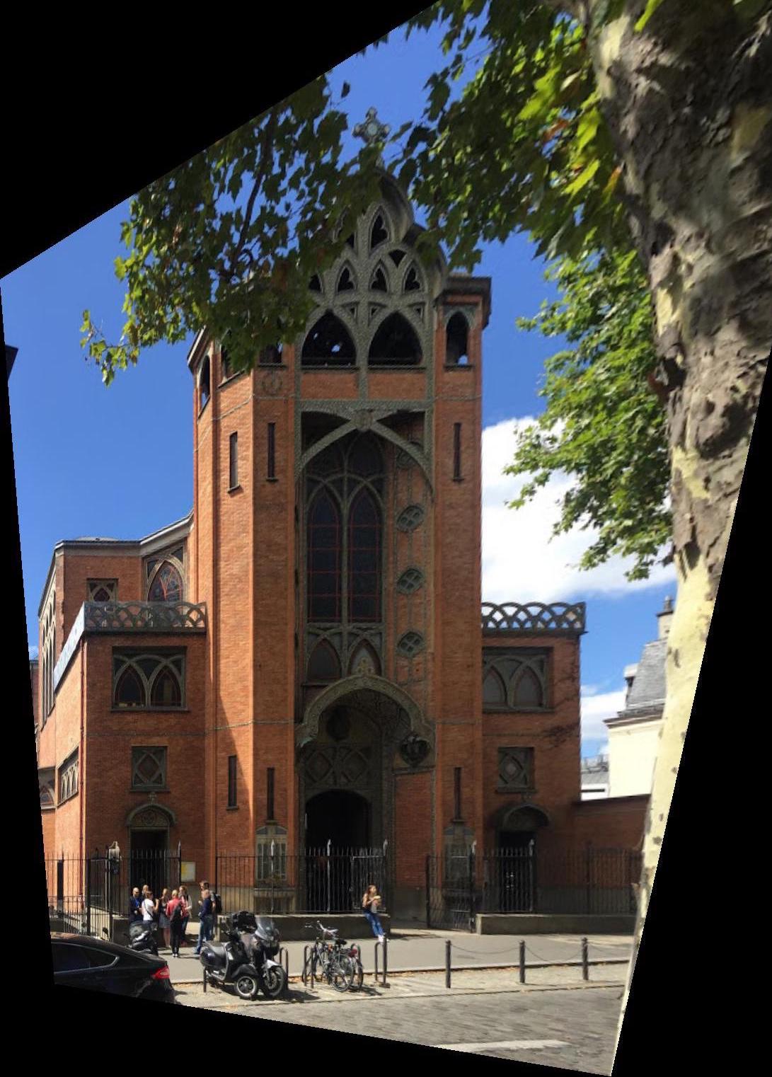 On the left is the original image, in the middle is after a homographic rectification is applied, and on the right is the cropped final image.