

For this project, I took pictures of a couple different scense with lots of overlapping content, and used a projective transformation to rectify them or stitch them together to form a mosaic
The results are shown below
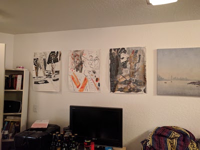
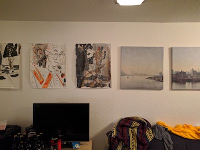
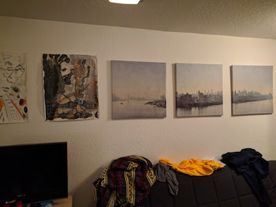
First, I went to shoot the images. It was very important to keep the center of projection the same for all images, so I tried to rotate the camera around the lens.
|
|
|
|
|---|---|---|
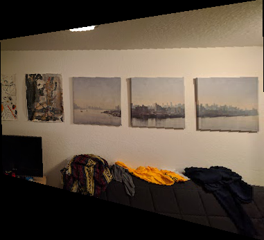
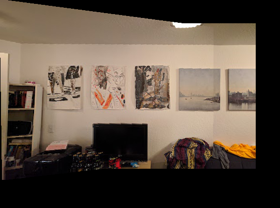
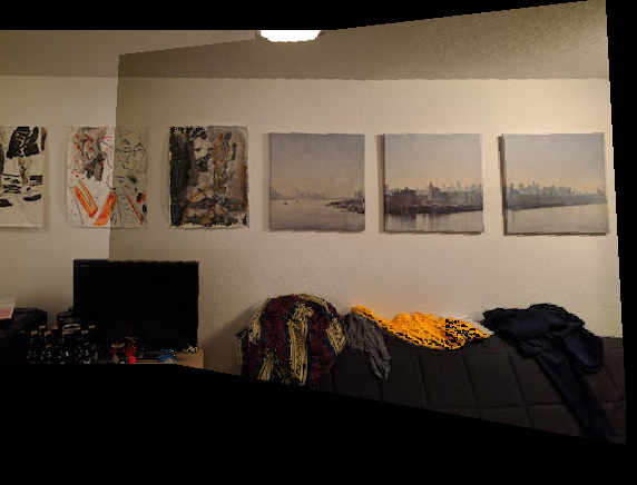
| Interior of my Friend's Apartment | ||
|
|
|
|
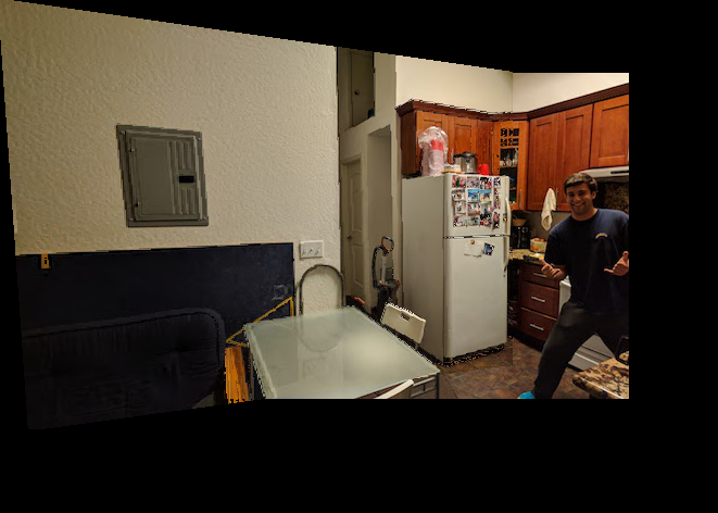
| My Kitchen |
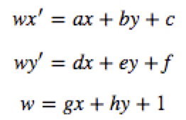
Next I needed to recover the homographies between the images. A homography has eight parameters we can solve for and is the transformation which transforms one image into the image plane of another. I first solved the equations below before continuing. To compute the matrix, I supplied a list of correspondance points for each image that I manually picked, and then used a least squares solver to find the homography. We were given that for points (x,y) in one image, and (x', y') in the target image, that:
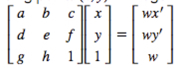
By matrix multiplication, we have:
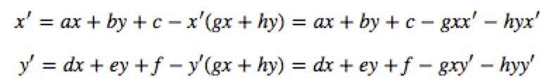
By solving for x' and y', we get the following:
Putting this back into matrix multiplcation form where h is a 1 dimensional vector, we get:
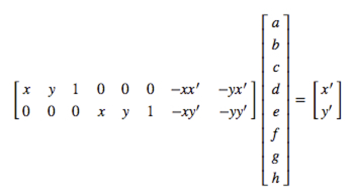
We solve this for every pair of correspondance points, and use the built in numpy least square solver to recover h.
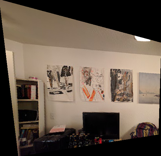
Now that we've solved for the homography, we can warp images from one viewpoint to annother. First, we calculate the bounding box of the resultant image by using the homography matrix on each of the corners, and keeping track of the max and min width and heights. Then, we use the matrix to fill the pixels of the resulting image to create the warp. Here are a couple examples:
|
|
|
|---|---|
| Original Image | Rectified to TV plane facing us |
|
|
|
| Original Image | Rectified to painting plane facing us |
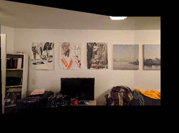
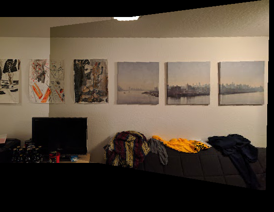
After rectifying, the next task was to actually blend two images together into a mosaic. I warped one image into the plane of another and then blended the result together at the corresponding levels to create a panorama. \n Three results are shown below:
|
|
|
|
|---|---|---|
| Original Images | ||
|
|
|
| Left and Center Mosaic | Center and Right Mosaic | |
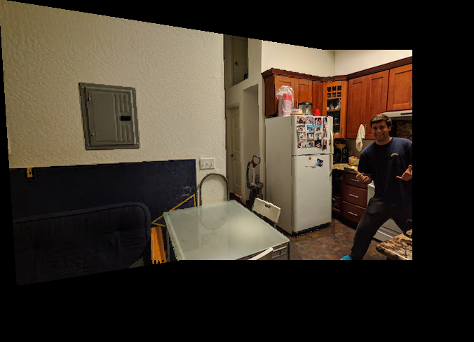
|
|
|
|
| Original Images | ||
|
||
| Resultant Kitchen Mosaic |
The goal of the second half of the project is to automatically define correspondance points instead of having to manually define them. Corners are automatically detected in images using the Harris corner detector, and later filtered with the ANMS algorithm. Feature descriptors are then extracted from the resultant points, and matched across the two images. These matched pairs are then used to compute a homography by the RANSAC algorithm. After automatically computing the resultant homography, we pass this homography to code from Part 1 to stich a panorama.
We first try to detect possible correspondance points using the Harris corner detection algorithm. This produces quite a few too many points so we use the ANMS algorithm to suppres the amount of corners. Results of each algorithm are shown below:
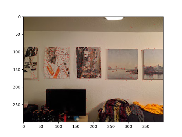
|

|
|---|---|
| Harris Points | Corner Points after ANMS |
You can see that ANMS filters out points and evens out the distribution throughout the picture. ANMS works by searching for the radius in which the point is a local maximum, and then taking the top points with the largest associated radii
Once we have the output of ANMS, we extract image descriptors from each point. These will eventually be used to match points between two images. To compute a point's descriptor, a 40x40 square centered on the point is extracted, blurred and downsampled to 8x8 via imresize, and then bias and gain normalized. For feature matching, we aim to match these features between the two images. Each feature in the first image is then matched with set of features in the other image. The SSD between every feature from the first image and every feature in the second are computed. We then take the ratio of the distance to the nearest neighbor to the distance to the second nearest neighbor and threshold it at a value of 0.4 to filter out invalid feature matches.
With possible features now matched, the final step is to compute the most likely homography. Since least squares matching is quite sensitive and the matches often times have errors, it is necessary to compute homography estimates in a more robust way. We use the RANSAC algorithm to achieve this. Four matches are sampled at random and a homography is computed. This homography is then used for all features and we calculate the result against the true values of the features. We then threshold the euclidean distance between the points, and keep track of the number of inliers that lie within the threshold. We run this process 10,000 times and use the homography that resulted in the most amount of inliers. This final homography is used for the image warp from part 1
|
|
|---|---|
| Autostiched Result | Manually Defined Result |
|
|
| Autostiched Result | Manually Defined Result |
|
|
Autostiched Result | Manually Defined Result |