Overview
In this project, we combine multiple images by projective warping and blending to create an image mosaic.
Homographies
I calculated the homography matrix using the 2 equations Hp = p' and Ah = b, where H is the transformation matrix, p , p' are vectors of (x, y) points, h is a vector of 8 degrees of freedom (a, b, ..., h), and A is the matrix I derived so that x' = ax + by + c - gxx' -hyx' and y' = dx + ey + f - gxy' - hyy'.
Image Rectification
Using the homography matrix,
I was able to "rectify" images so that the images would be warped so that planar surfaces would be frontal-parallel.
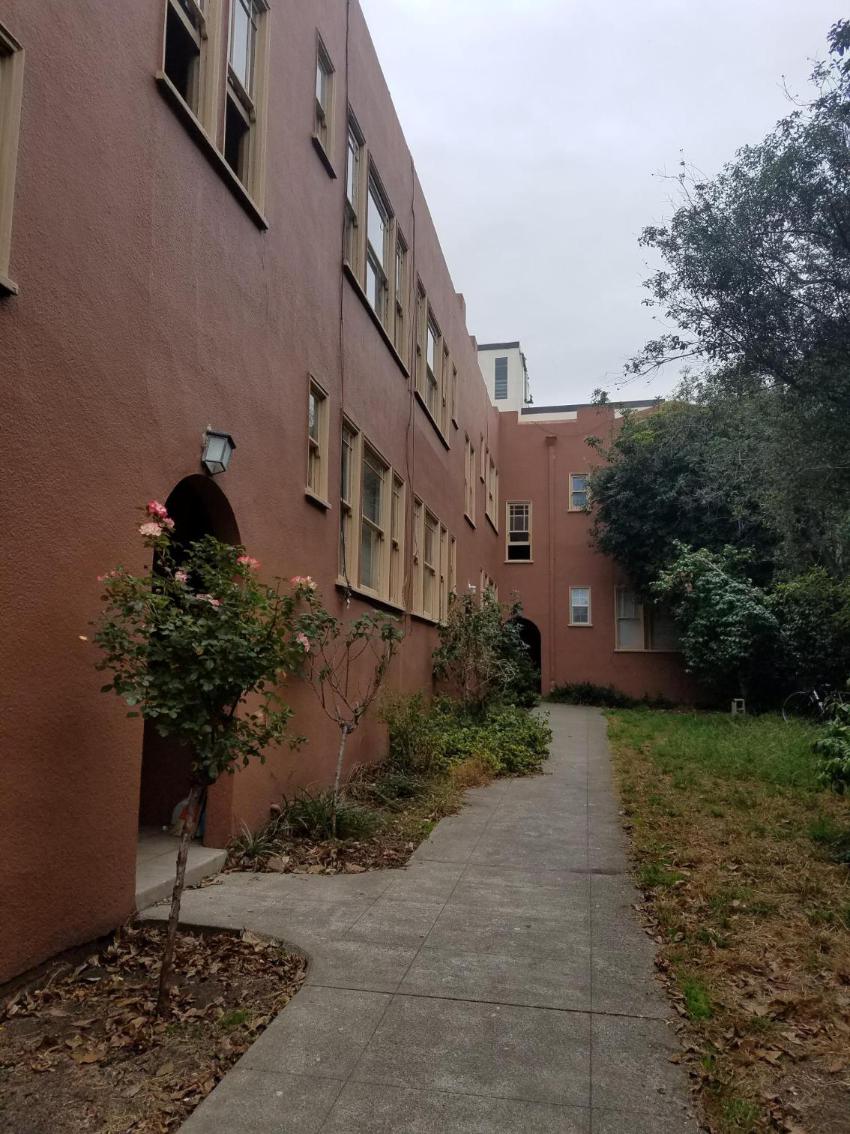 Original
|
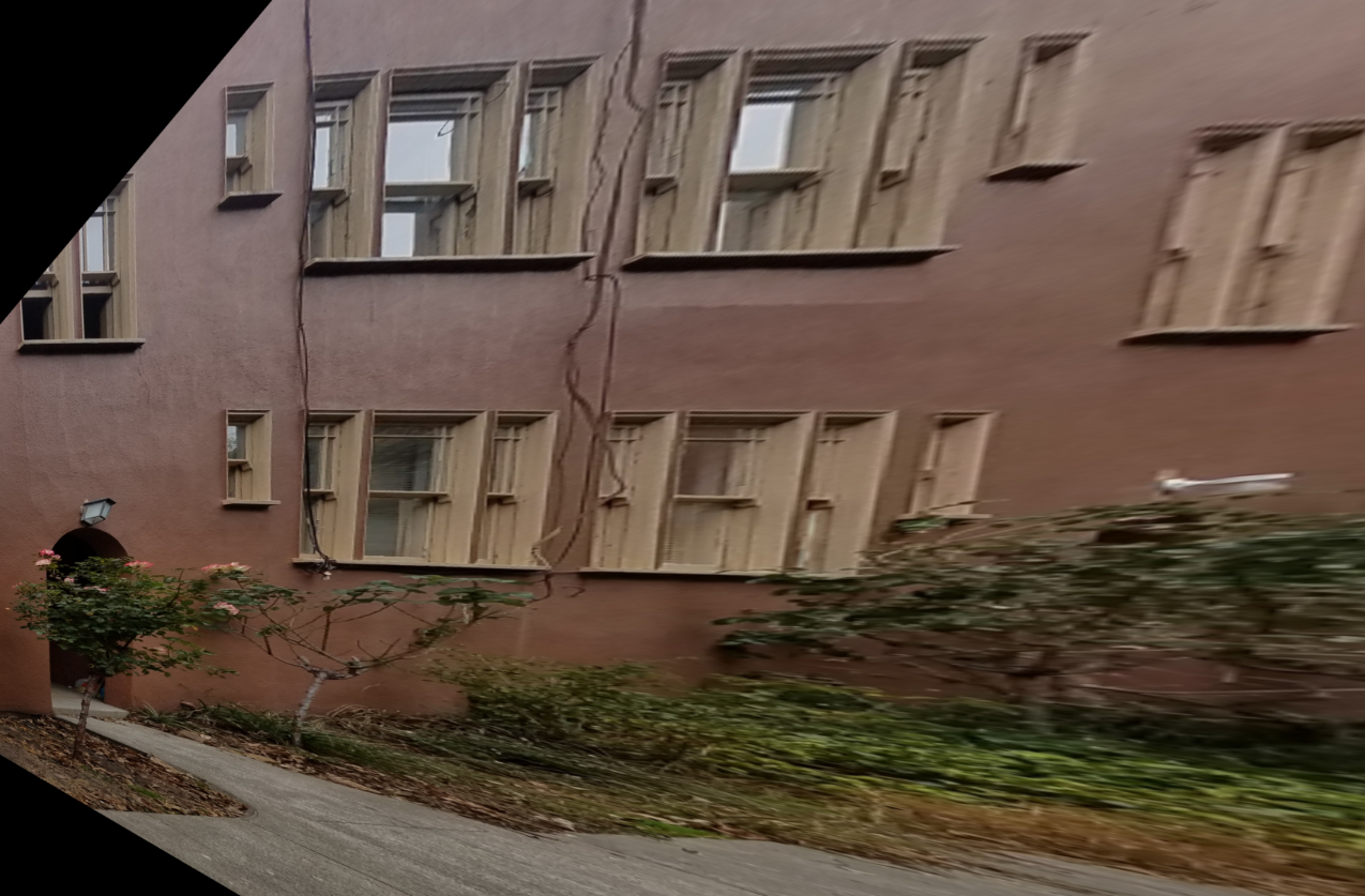 Recitifed to window
|
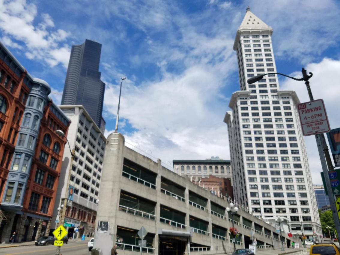 Original
|
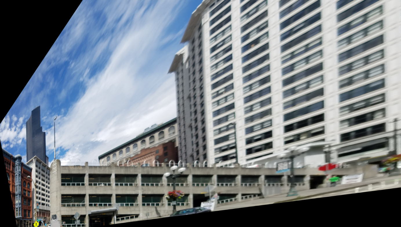 Recitifed to parking lot window
|
 Original
|
 Recitifed to box
|
Mosaics
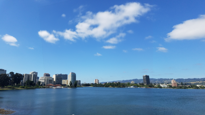
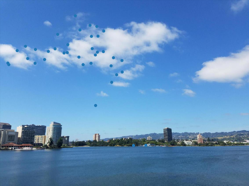
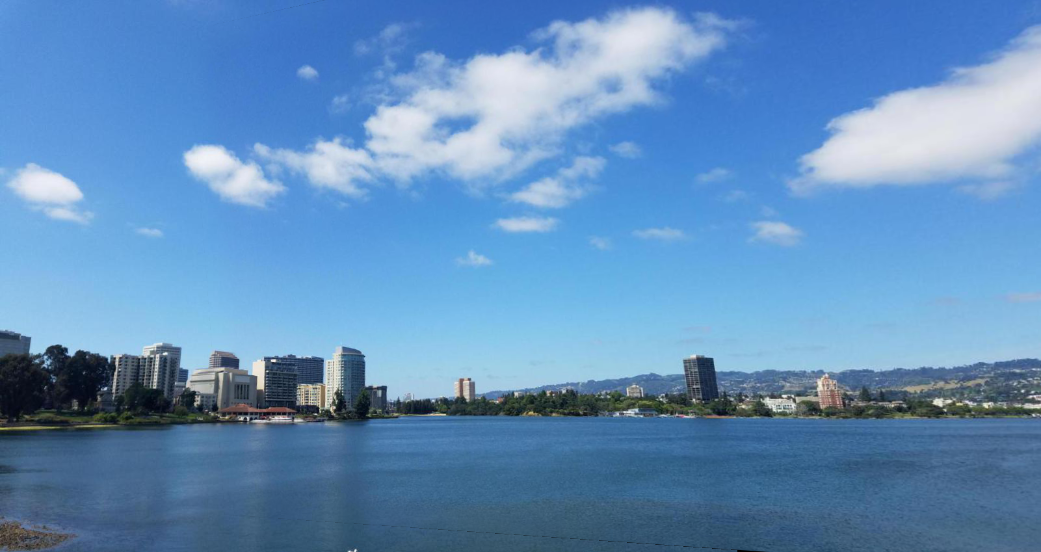
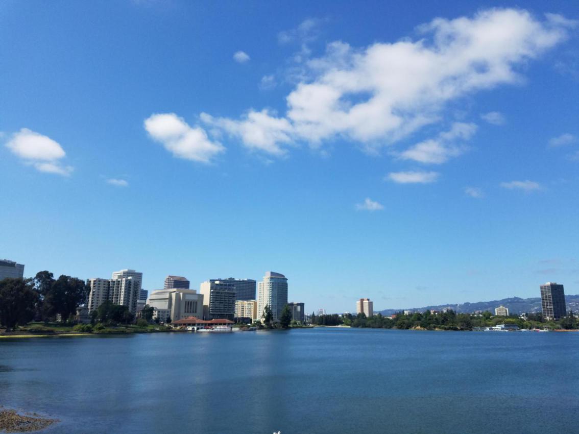 Oakland image 1
|
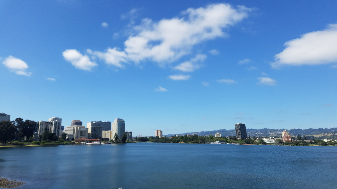
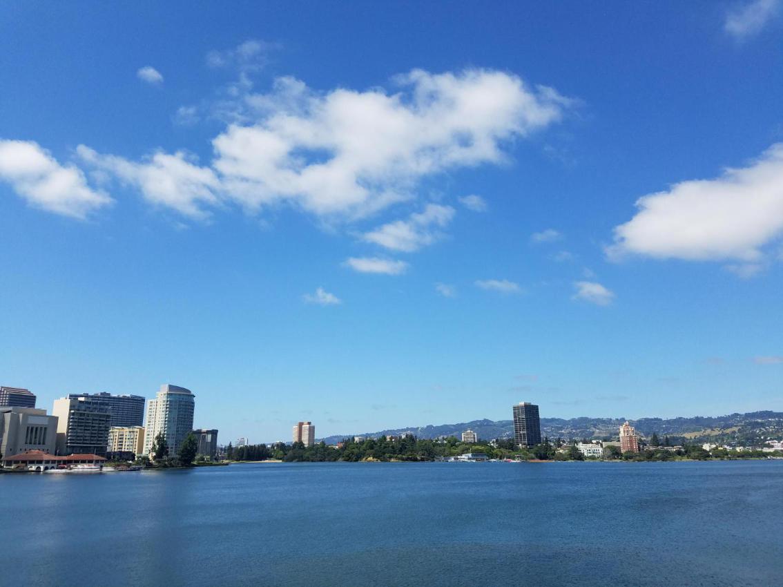 Oakland image 2
|
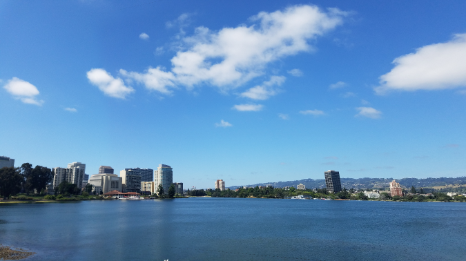
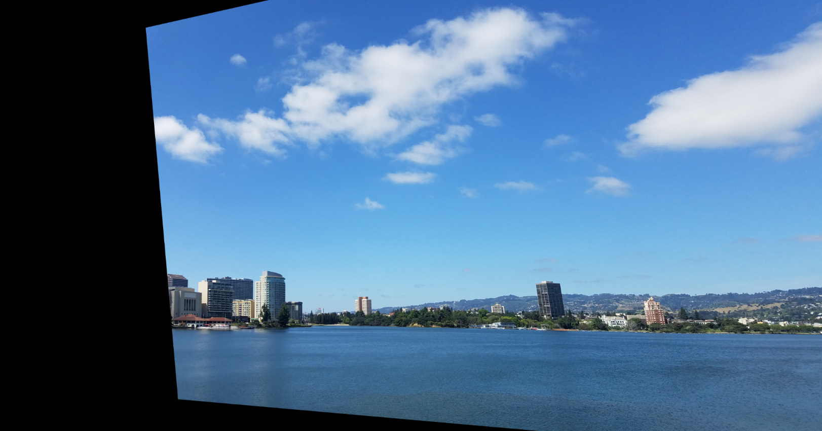 Oakland image 2 warped
|
 Average blending
|
 Linear blending
|
 Laplacian blending
|
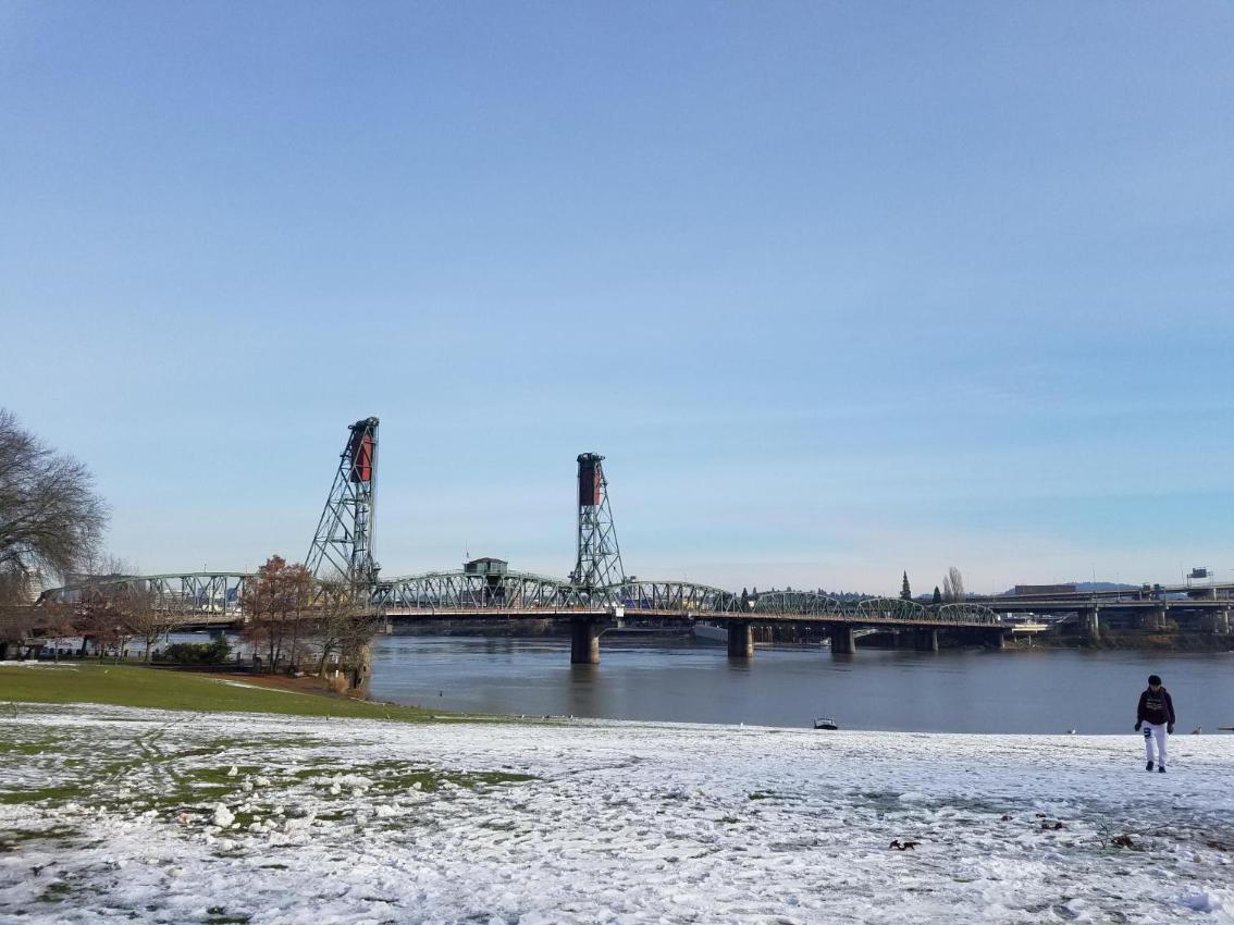
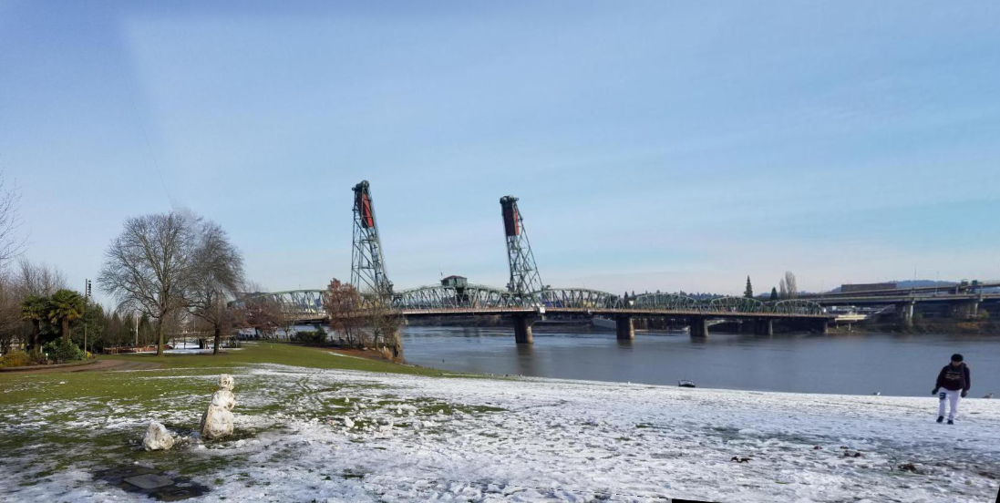
 Portland image 1
|
 Portland image 2
|
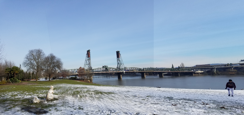 Average blending
|
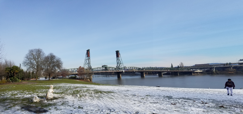 Linear blending
|
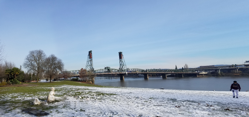 Laplacian blending
|
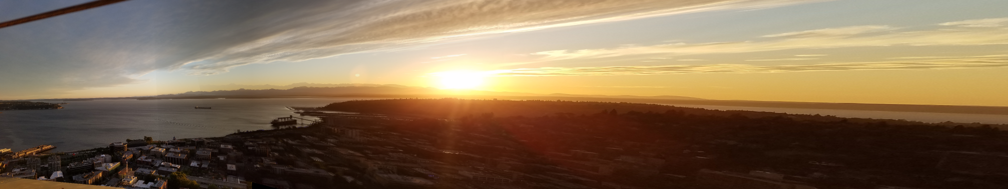
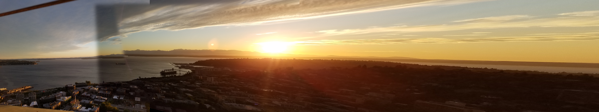
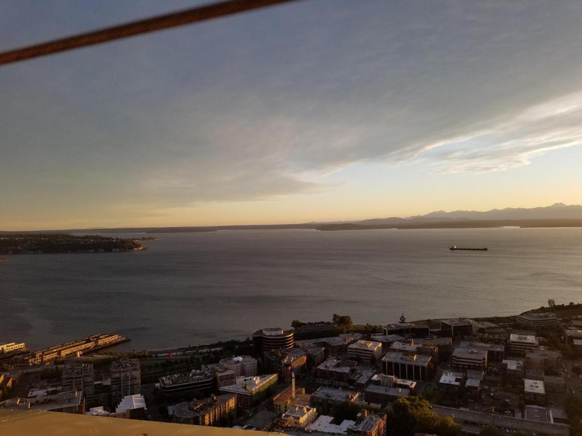 Seattle sunset image 1
|
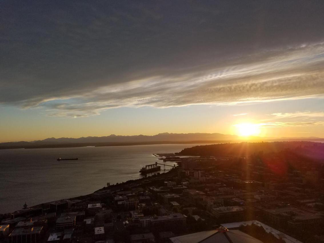 Seattle sunset image 2
|
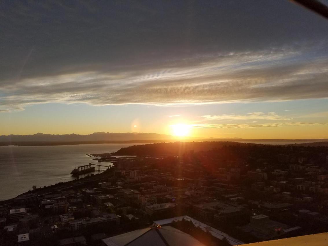 Seattle sunset image 3
|
 Average blending
|
 Linear blending
|
 Laplacian blending
|
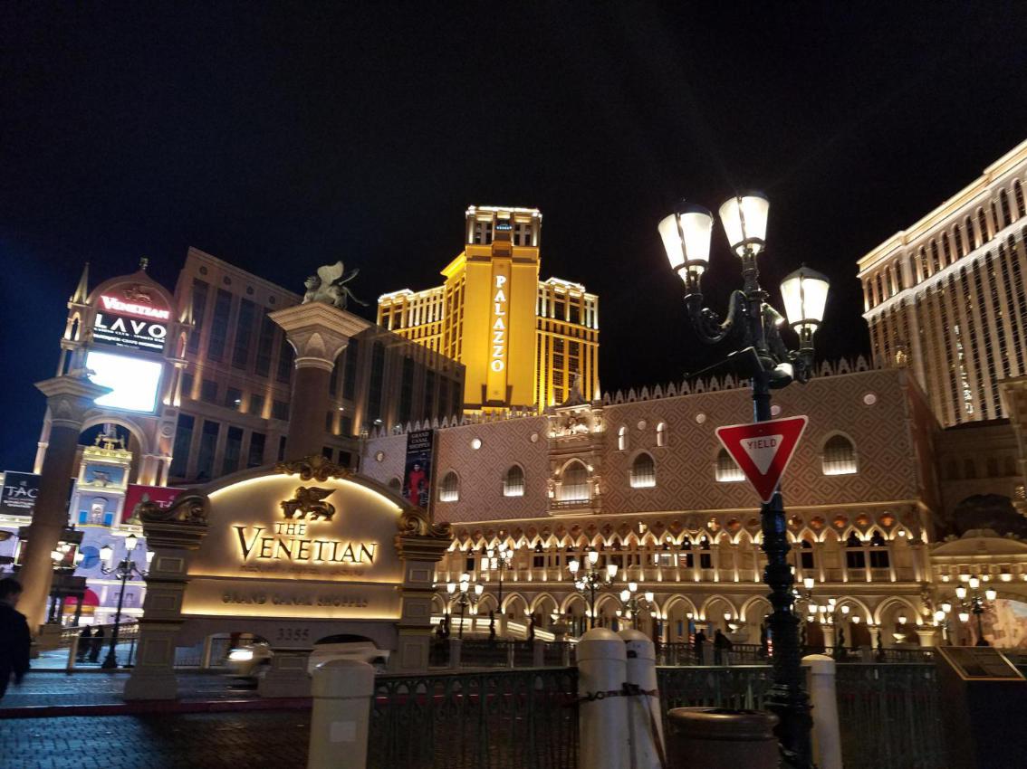 Las Vegas image 1
|
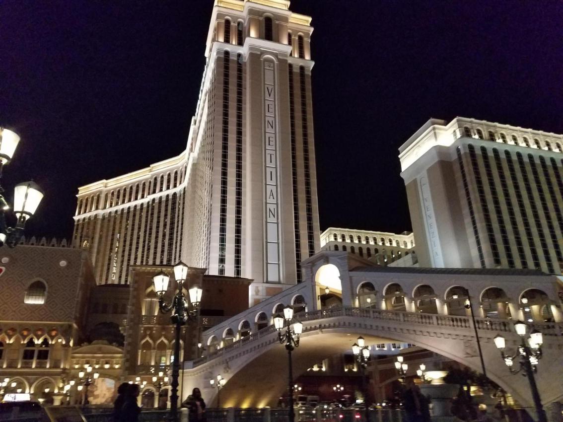 Las Vegas image 2
|
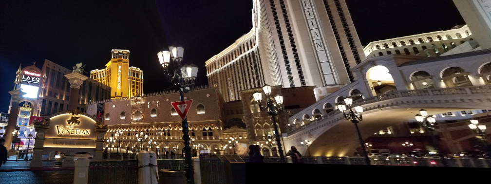 Average blending
|
 Linear blending
|
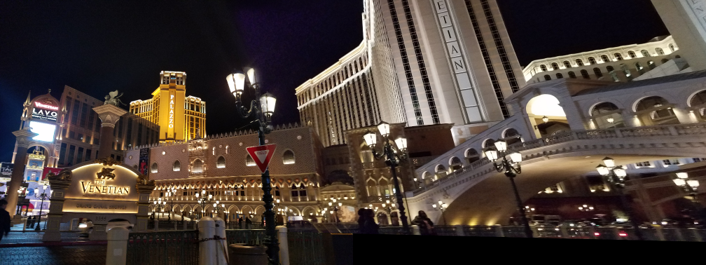 Laplacian blending
|
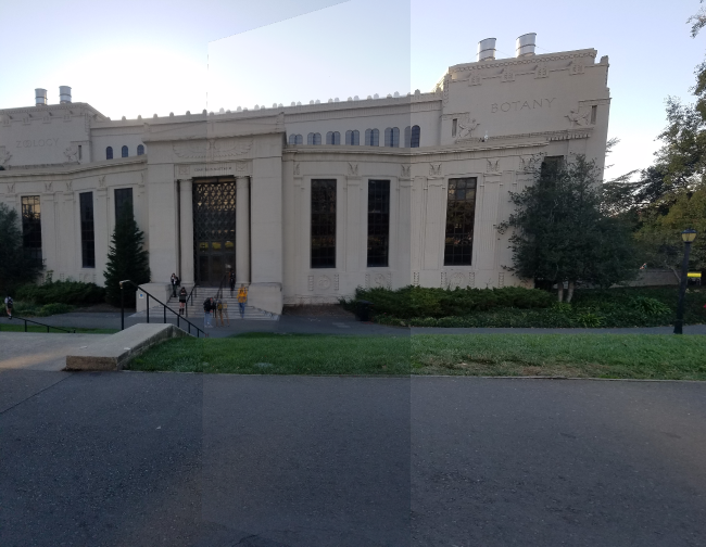
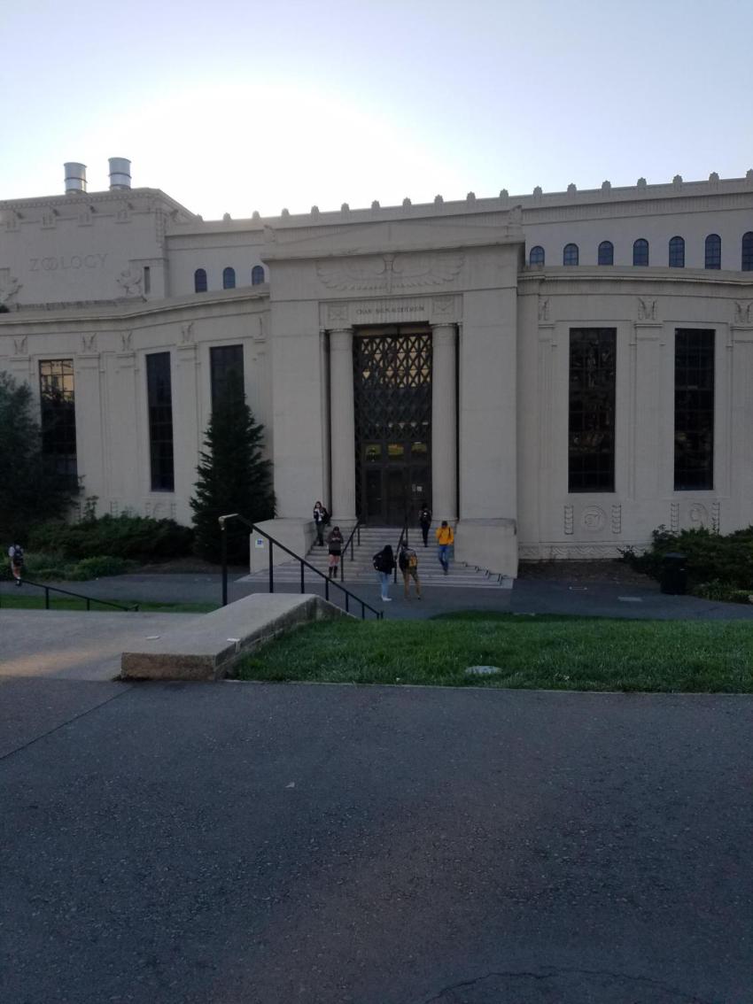 VLSB image 1
|
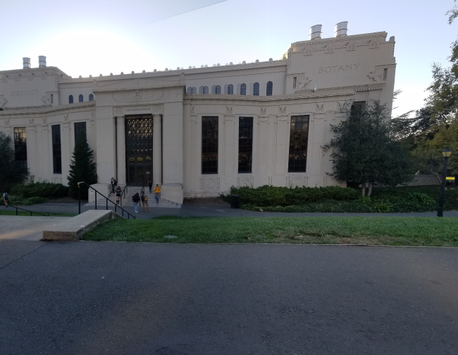
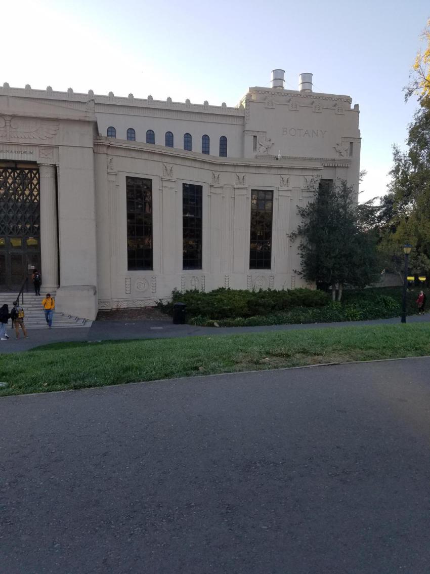 VLSB image 2
|
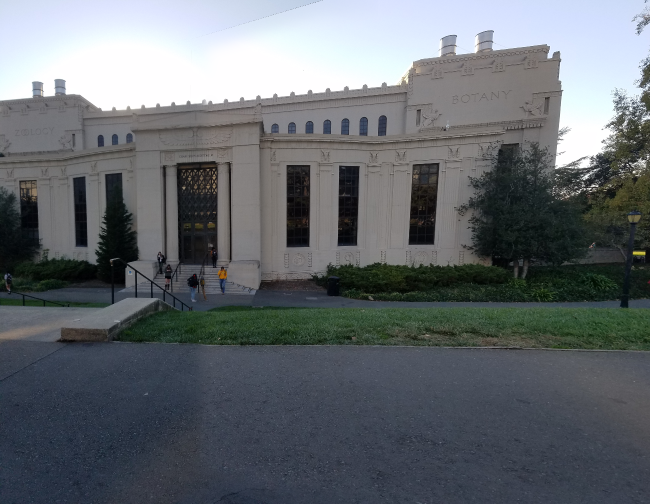
 Average blending
|
 Linear blending
|
 Laplacian blending
|
Summary
When blending the images together, Laplacian blending works best when the images' colors are similar.
It also works great in getting rid of ghosting, so the resulting images are sharp compared to other blending methods.
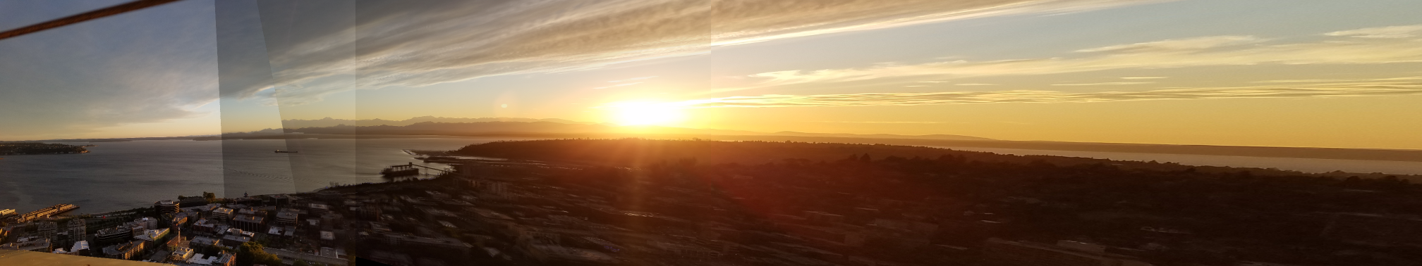
But linear blending works best when the colors of the images differ greatly, like in the Seattle sunset picture.
In the VLSB photo, in the linear blended image, there is a litte ghosting on the windows at the top but the color transitions very smoothly.
On the other hand, with Laplacian, the image is sharp but half of the building is a different color from the other half.
B & W -Blending and Compositing (from lecture slides)
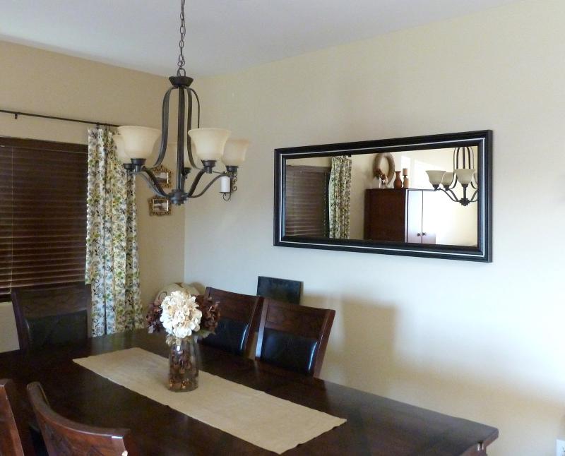 Mirror
|
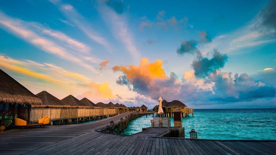 Maldives
|
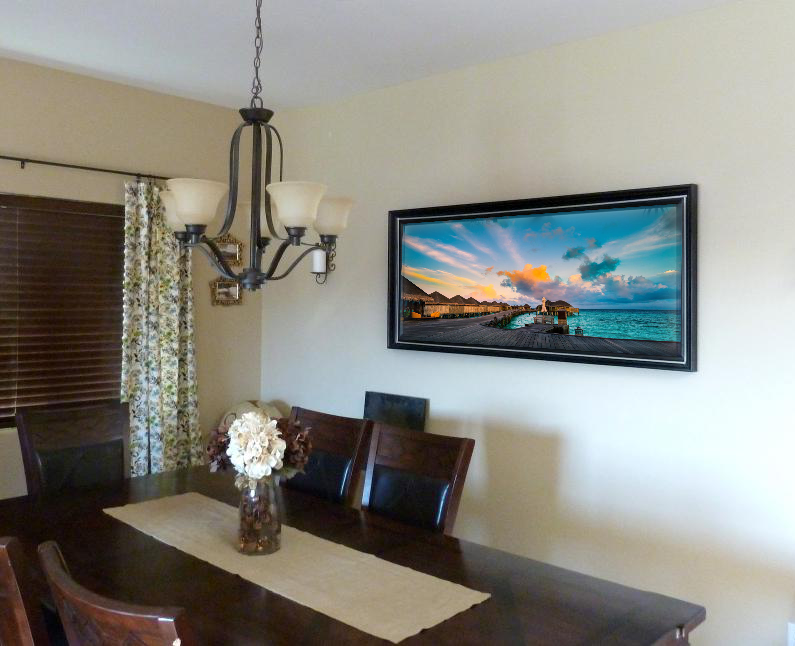 Result
|
|
VLSB
|
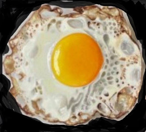 Egg
Egg
|
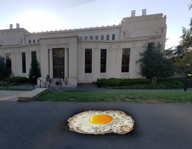 Another composite
|
Part B
Harris Corner Detector & Adaptive Non-Maximal Suppression
For Harris corner detection, I used the code provided and because the function found way too many points, I used adaptive non-maximal suppression to get evenly distributed features.
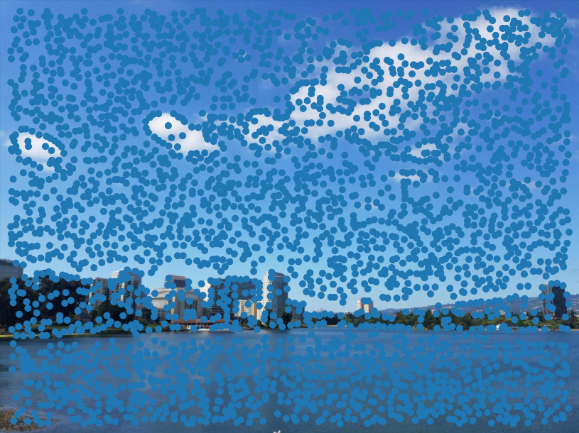 Harris corners
|
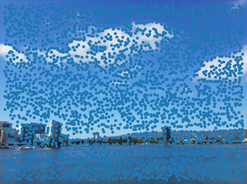 Harris corners
|
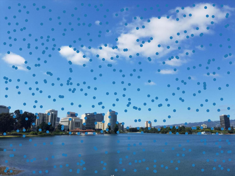 After ANMS (500 features)
|
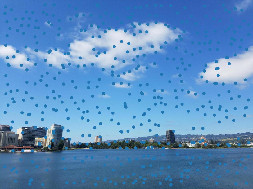 After ANMS (500 features)
|
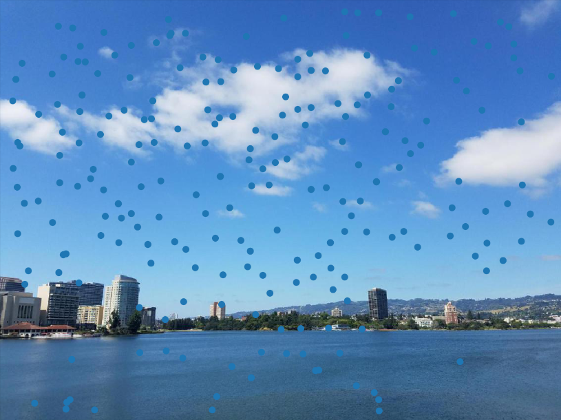
Feature Matching
After getting all the features, I matched the features from image 1 to features in image 2 by getting a 40x40 window, downsampling to 8x8 and calculated the distance between all points. Then I for each feature in image 1, I stored the closest features from image 2. And I filtered the features that didn't have close matches using the Lowe threshold (1-NN / 2-NN > .6).
 Matched Features
|
 Matched Features
|
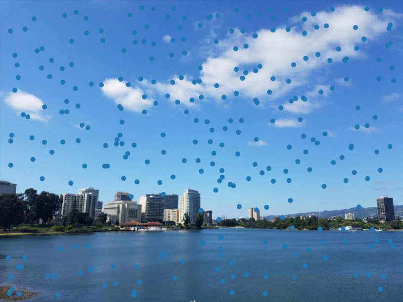 Matched 291 Features
|
 Matched 291 Features
|
RANSAC
However, since these matched features are not 100% accurate and least squares is not robust to outliers, I used RANSAC to compute a robust homography estimate.
It works by randomly selecting 4 points to use to compute homography H.
Then you compute the number of inliers and this is repeated for x number of times.
The largest set of inliers are kept and used to compute a new homography to create your mosaic.
 37 Matches Image 1
|
 37 Matches Image 2
|
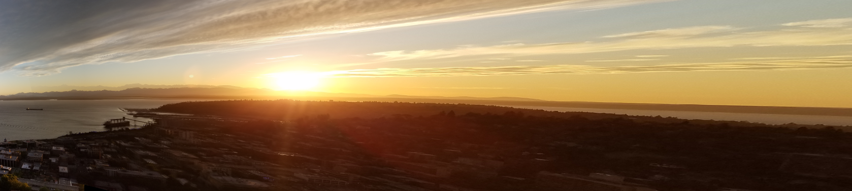
 Resulting Panorama
|
|
Panorama with hand chosen features
|
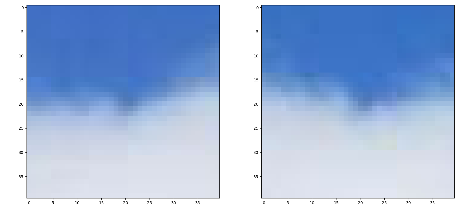
 Seattle 2 + 3 - Automatic
|
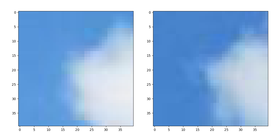
 Manual
|
 Automatic
|
|
Manual
|
The automatically aligned panorama is slightly less blurred in the overlapping areas. And even though only the clouds were matched in the first image, the panorama still came out good.
The automatic method also distorts the images less.
Things I Learned
Automatically detecting features is a great way to align images but doesn't always work well if the detector can't match features well.
Also, in RANSAC, increasing the epsilon value can sometimes help in finding better homographies. But if you increase it too much, it'll use inaccurate features, which will make your panorama worse.