Part A Overview

The goal of this project is to automatically stitch together images, much like the concept of taking a creating a panorama using your phone by taking multiple pictures. To start, we would first manually define corresponding points to find the homographies and use them to warp an image to match the other. However, the minor differences in lighting and texture may prevent it from looking authentic. By mosiacing the images, we can make it look more seamless. This setup helps in starting the autostitching in part B.

Shoot the Pictures

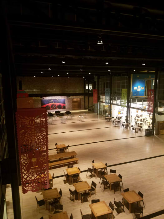
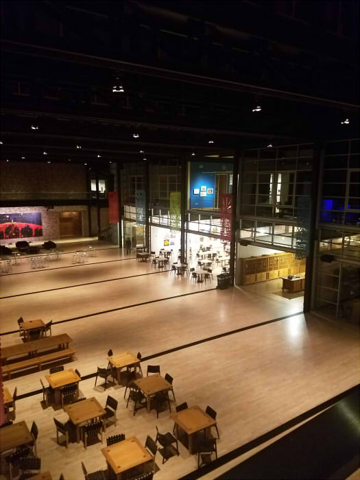
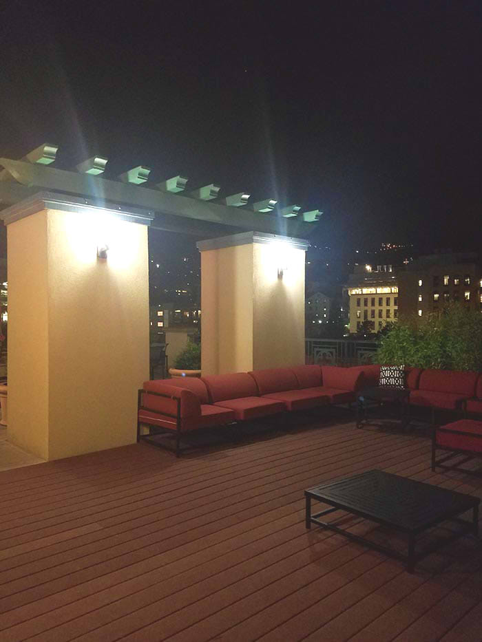
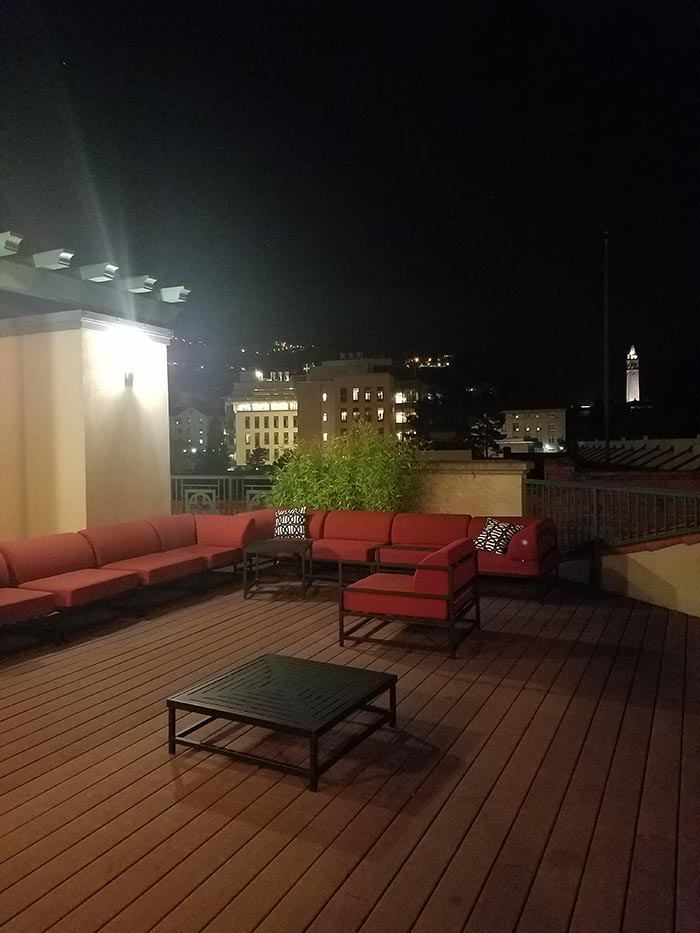
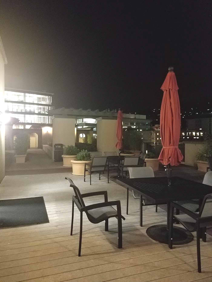
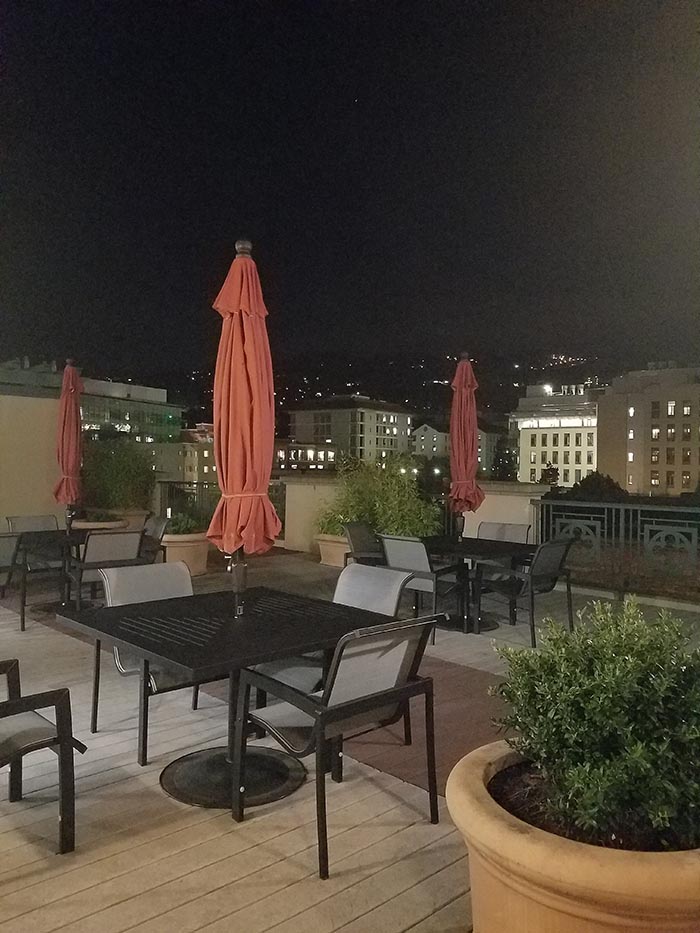
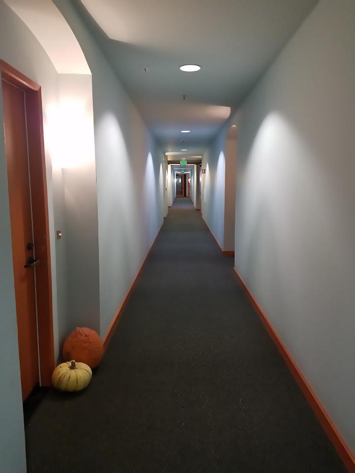
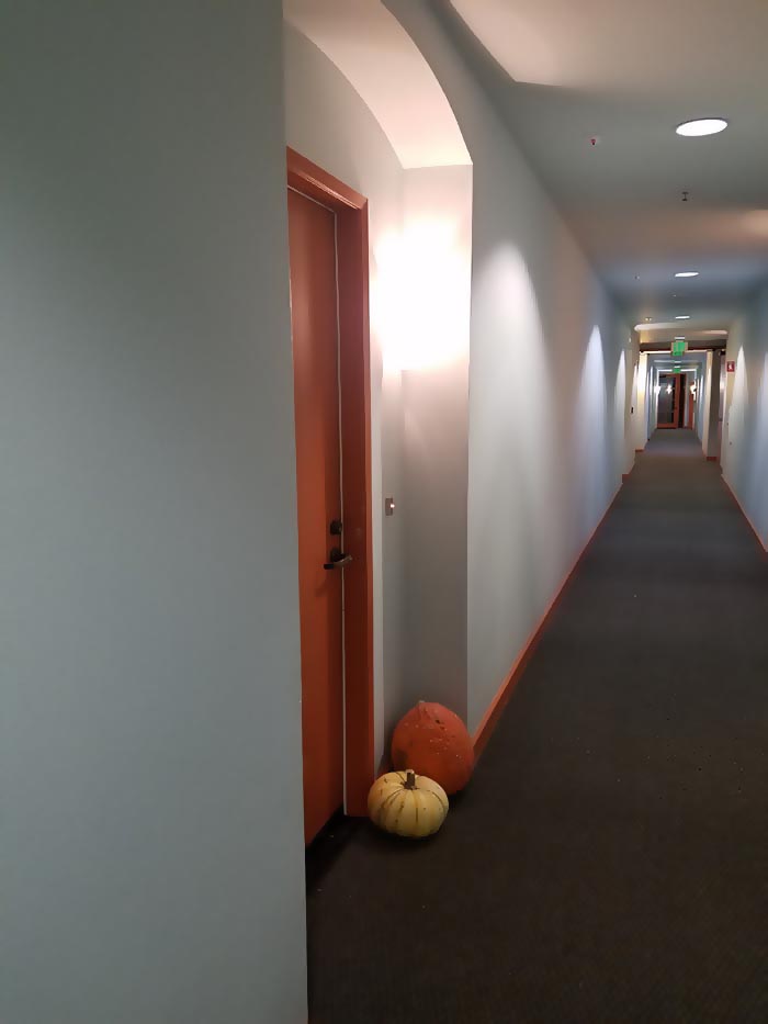
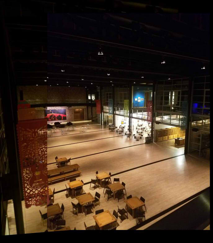
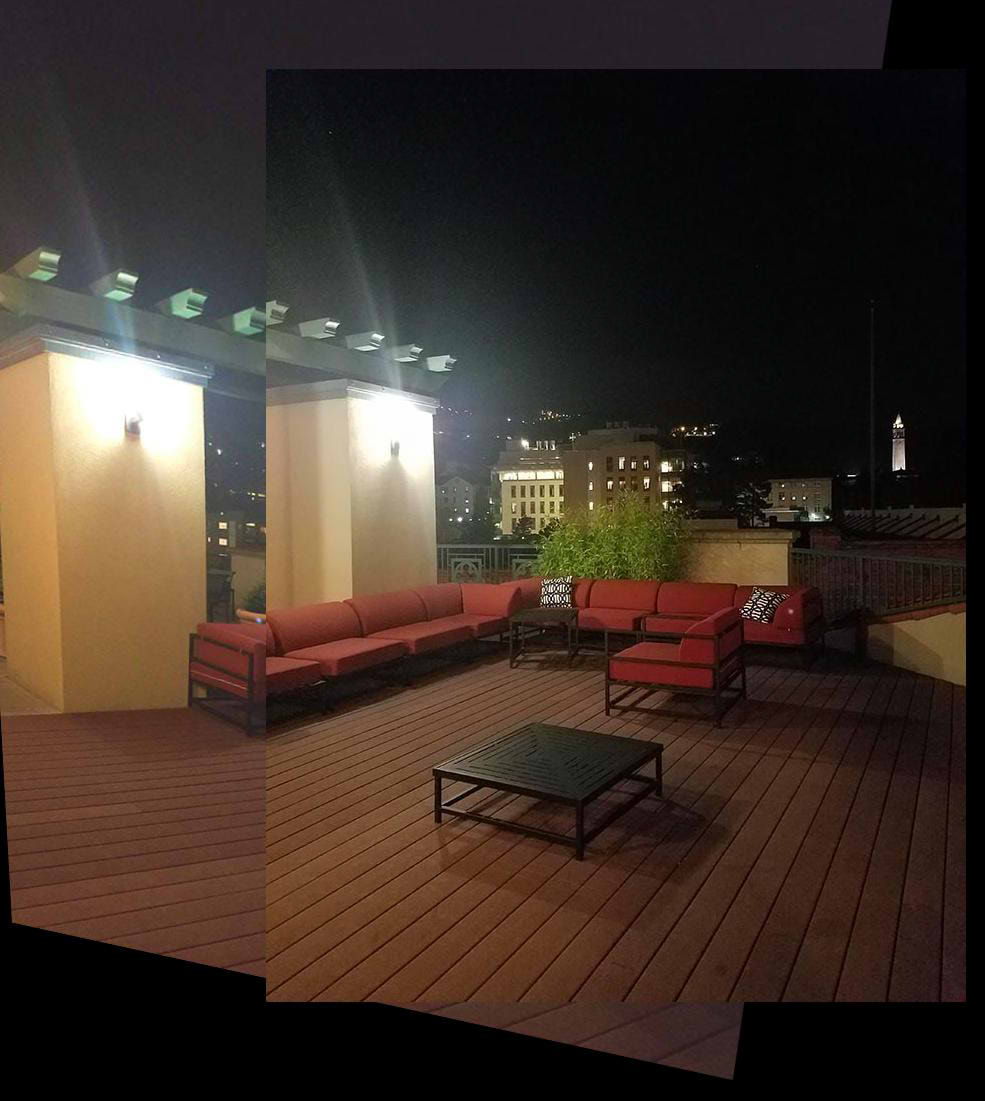
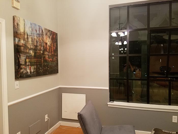
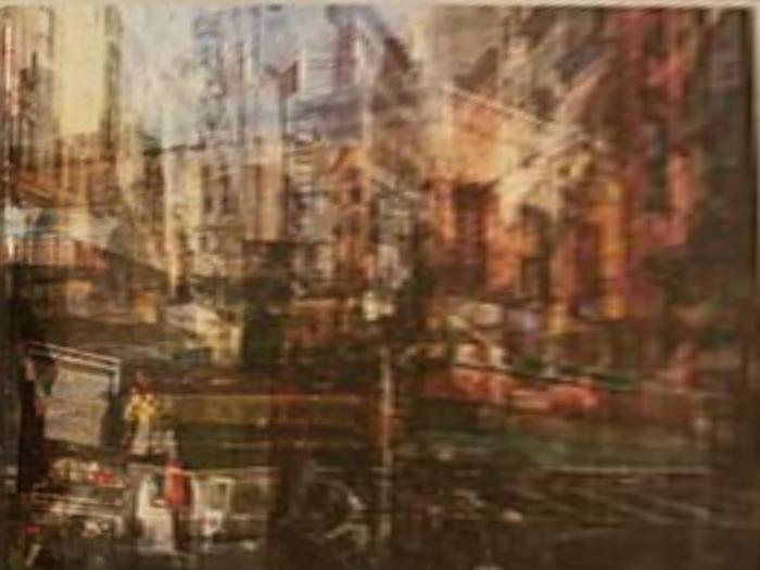
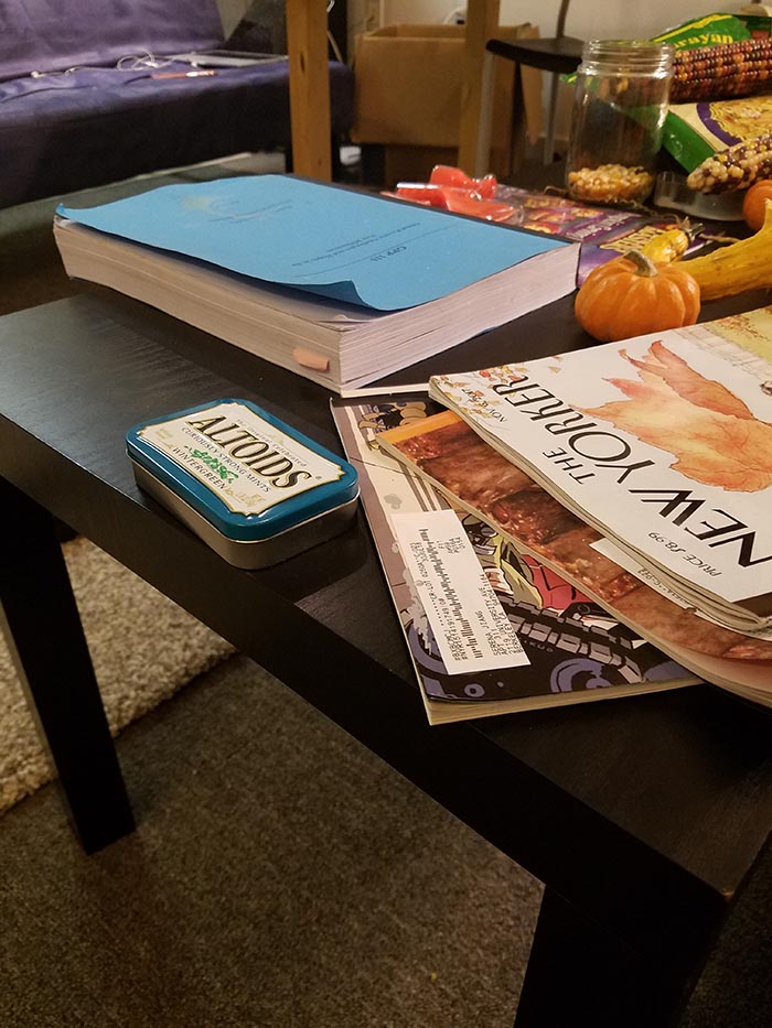
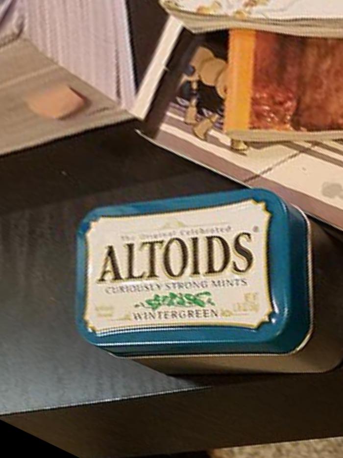
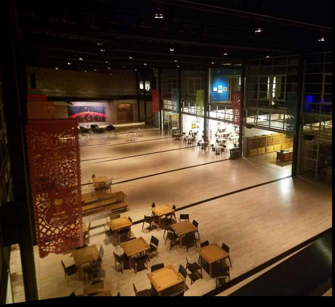
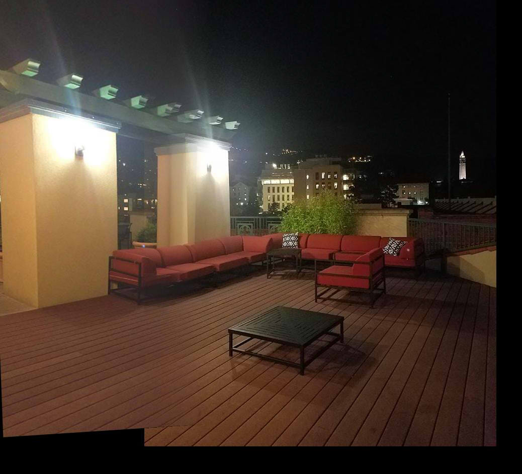
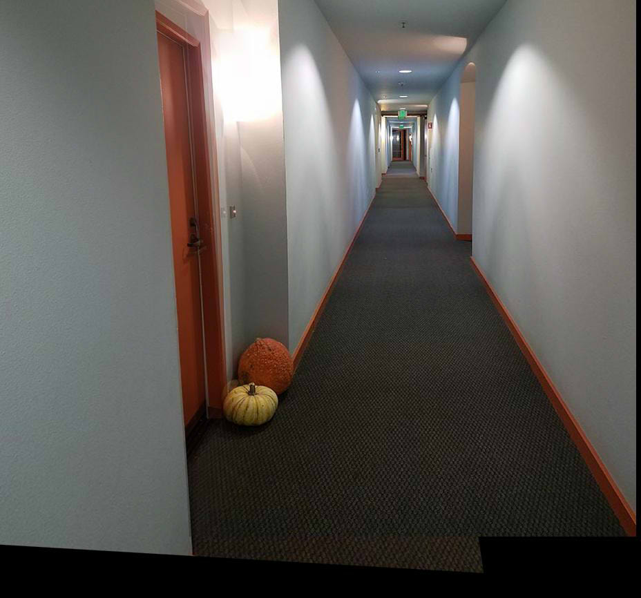
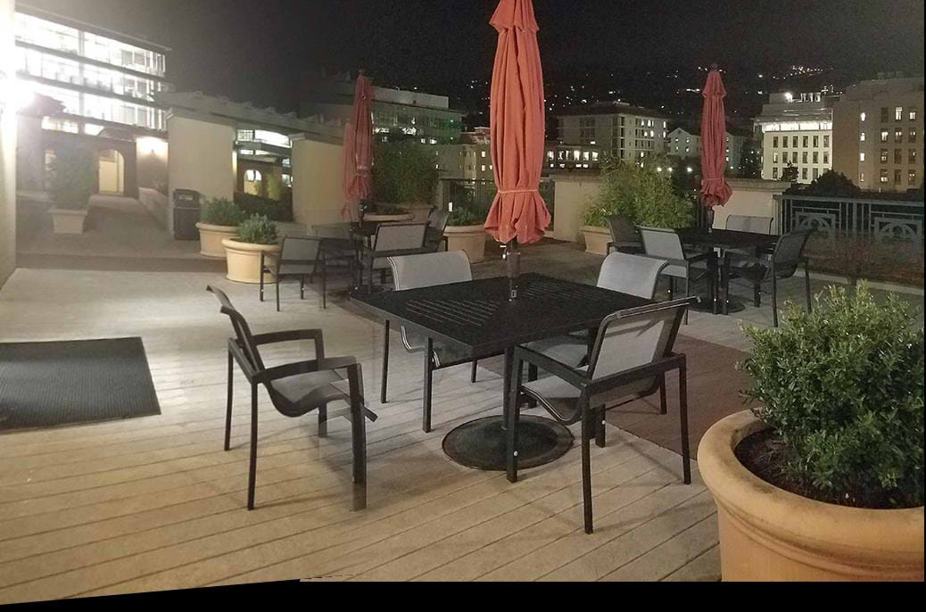
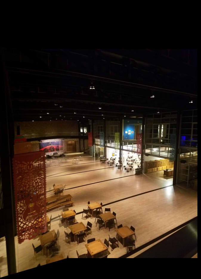
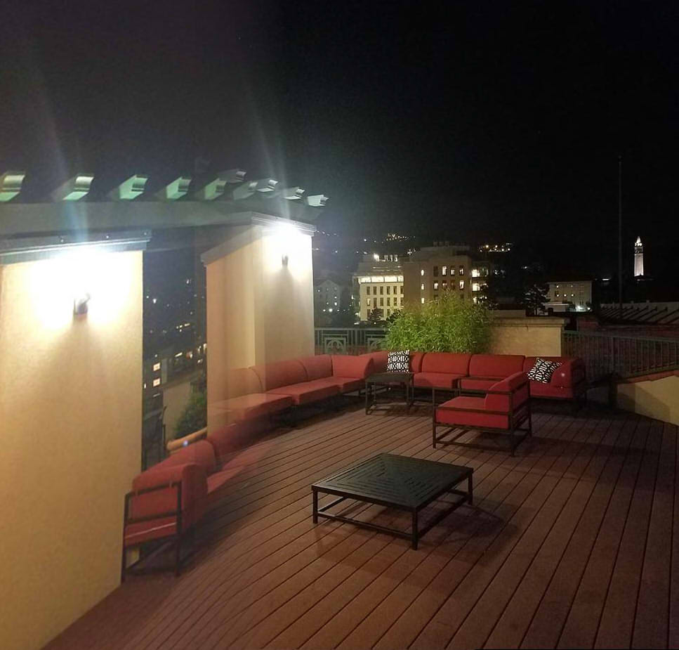
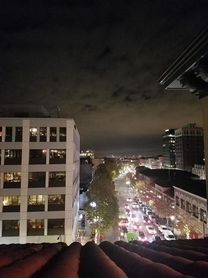
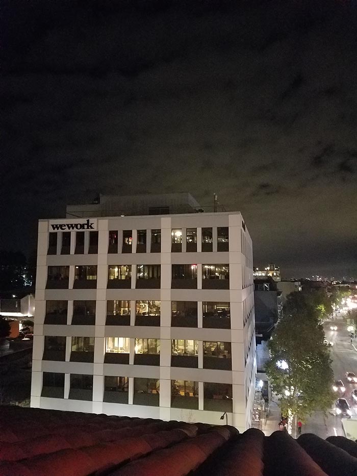
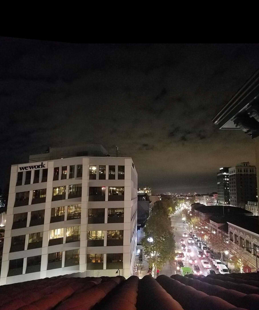
These are a couple images I shot from my phone. Since I didn't have a tripod, I tried my best to rotate the camera in place.

Recover Homographies

To recover the homography, we need many points and the forumla below:

$H = \begin{bmatrix}a & b & c \\ d & e & f \\ g & h & 1\end{bmatrix} \longrightarrow \begin{bmatrix}a & b & c \\ d & e & f \\ g & h & 1\end{bmatrix} \begin{bmatrix}x \\ y \\ 1\end{bmatrix} = \begin{bmatrix}wx' \\ wy' \\ w\end{bmatrix}$

We let $H$ be the homography $(x, y)$ be the the point from the image we want to warp, $(x', y')$ be the point on the image we want to match,and $ w $ be a scalar

We can then put it in the form of $Ax=b$ so that we can solve for $x$. We can also solve for multiple points to increase accuracy.

$\begin{bmatrix} x_1 & y_1 & 1 & 0 & 0 & 0 & -x_1x_1' & -y_1x_1' \\ 0 & 0 & 0 & x_1 & y_1 & 1 & -x_1y_1' & -y_1y_1' \\ x_2 & y_2 & 1 & 0 & 0 & 0 & -x_2x_2' & -y_2x_2' \\ 0 & 0 & 0 & x_2 & y_2 & 1 & -x_2y_2' & -y_2y_2' \\ x_3 & y_3 & 1 & 0 & 0 & 0 & -x_3x_3' & -y_3x_3' \\ 0 & 0 & 0 & x_3 & y_3 & 1 & -x_3y_3' & -y_3y_3' \\ \vdots & \vdots & \vdots & \vdots & \vdots & \vdots & \vdots & \vdots \\ x_n & y_n & 1 & 0 & 0 & 0 & -x_nx_n' & -y_nx_n' \\ 0 & 0 & 0 & x_n & y_n & 1 & -x_ny_n' & -y_ny_n' \\ \end{bmatrix} \begin{bmatrix}a \\ b \\ c \\ d \\ e \\ f \\ g \\ h \end{bmatrix} = \begin{bmatrix}x_1' \\ y_1' \\ x_2' \\ y_2' \\ x_3' \\ y_3' \\ \vdots \\ x_n' \\ y_n' \\ \end{bmatrix}$

Warp the Images

We can warp the image much like in project 4 by using inverse warping. While I have implemented my own warping function, I recently found in piazza that we can use sk.transform.warp, which is much faster. I then mask the warped image and add it to the one we want to match. While things do match up, the seam seems pretty visible

Image Rectification

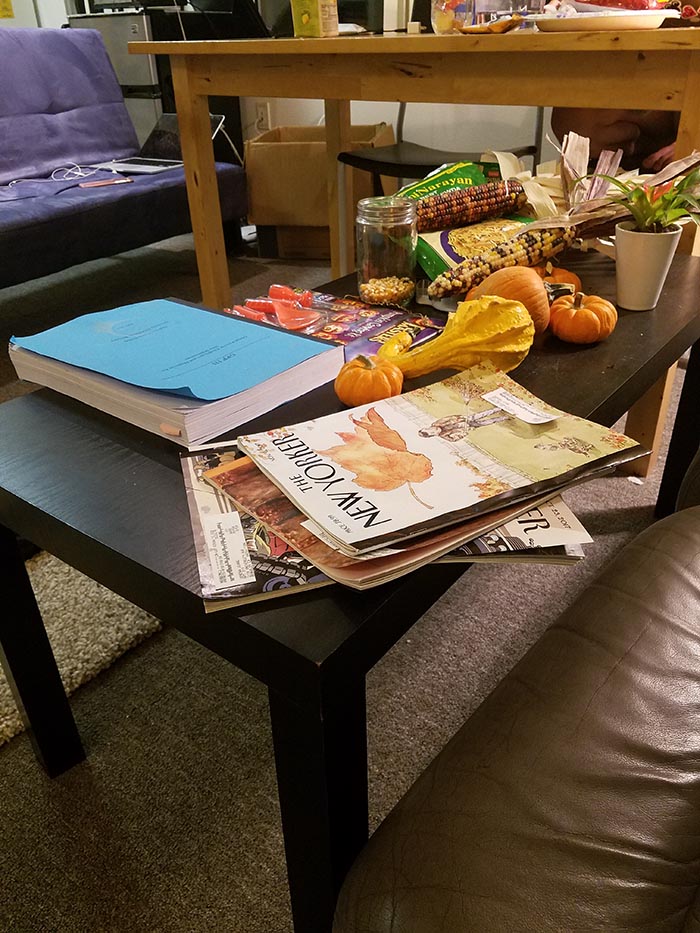
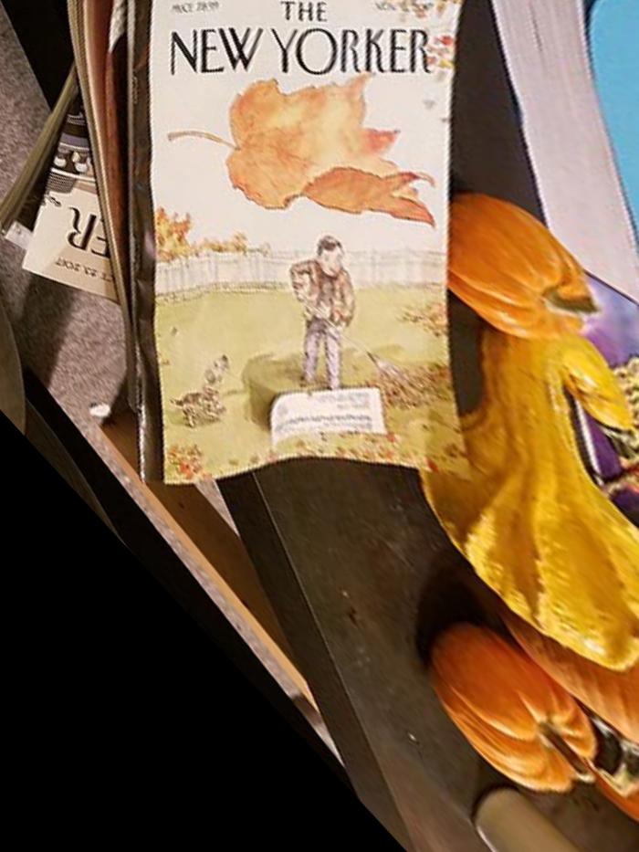
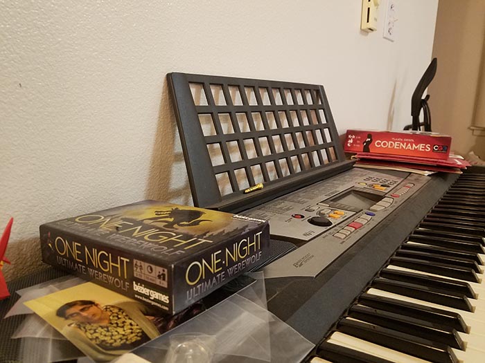
For image rectification, we only need 4 points to define the item we want and the plane we will project it onto. There only needs to be one image since we don't need to match it to anything other than a plane.

Blend the images into a mosaic

To get rid of the seam from before, we can blend the images to create a better mosaic. First we find the binary mask of the intersection. Then we weight the mask non-uniformly so that from right to left so that the drop-off is larger near the seam. Using the weighted mask, we can add the two images in the intersection each wth different weights, resulting in a gradual blend.

Tell us what you've learned

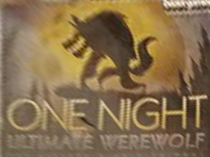
I've learned the impoprtance of taking pictures steadily since a good batch of my photos actually didn't work out too well. In terms of technical knowledge, I've learned a bit more abotu transformations and how to navigate around that especially since there were transformations into negative space that didn't translate well into image indices. And as always, I'm learning so many different applications through the functions we write. For example, we're using rectification as a warping check even when it can be an entirely different application (like replacing planar objects--switching the cover of a magazine with the cover of the board game).

Part B Overview

In this part, we use corner detection and feature matching in order to automatically stitch images together as opposed to our manual way of picking points in the previous part. While very useful, the results tend to vary depending on which points are picked and as a result which homography is favored.

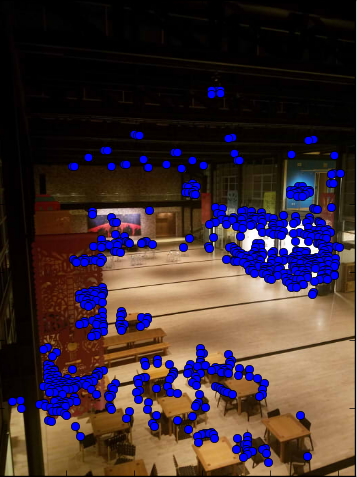
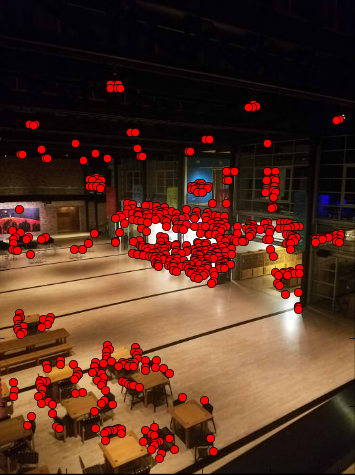
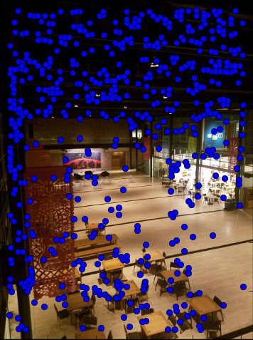
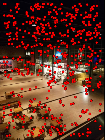
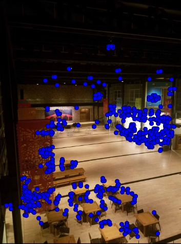
Detecting corner features in an image

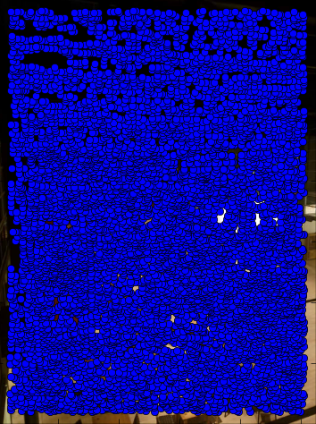
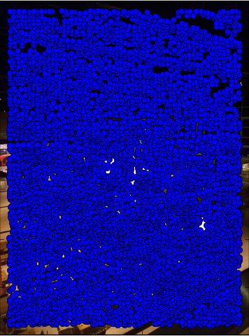
To detect the corners in an image, we use the Harris corner detection algorithm provided by harris.py to detect the corners in an image. I switched out peak_local_max (results seen in the first two images below) for corner_peaks (results seen in the last two images below) as I read that it was okay on Piazza and resulted in my code being overall faster.

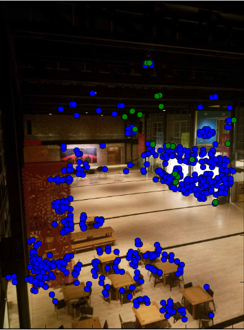
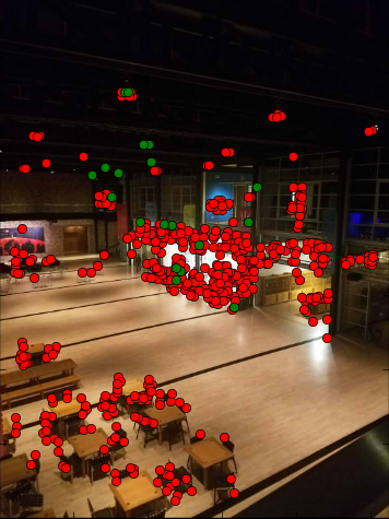
Extracting a Feature Descriptor for each feature point

We use the Adaptive Non-Maximal Suppression method as specified in the MOPS paper to select the strongest corners detected. For each Harris corner in one images, we find the distance from it to each of the Harris corners in the image we want to match it to. If it's strength is much stronger than the corner we compare it with, we take the distance and record it as the new minimum if it is smaller than it was previously. Afterwards, we select a number of points with the largest minimum distance. In this case, it is 500, which is seen to be more spread out with the peak_local_max in the Harris detector since there are more points needed. (The first two images below) In the current case (the second two images below), that is most of the points, which is why they are closer together.

Matching these feature descriptors between two images

For each point that we chose through ANMS, we take a 40x40 patch centered around the point to use as our feature descriptor. We then get rid of the high frequency and downsample it to an 8x8 patch.

Then, we calculate the distance between each feature and get the two nearest neighbors in terms of the distance. If the ratio between the nearest neight and second nearest neighter is smaller than a specifed threshold, we make the nearest neighbor we found a match.

Use a robust method (RANSAC) to compute a homography

To compute the homography, we use RANSAC to iterate through a good number of possibilites. We select 4 points at random and compute the homography. Then, we calculate the distance between them. If they are considered an inlier (their values are under a certain threshold), they are stored. Afterwards, we compare the inliers and for each homography and select the homography with the most.

Tell us what you've learned

Some of the results are not as good as manual picking and I completely understand why. When I was manually picking, I found it hard to pick points as well and because of that had to pick points over an over. This must be especially hard with the variance in my pictures and the precision I lost taking them from just my cellphone. I've learned that this project basically picks points better than I can. I guess I've learned that I'm very stupid, but that's really nothing new.