Wall Art
In this part of the project, we further explore the usages of image warping and the techinques of image mosaicing. To create an image mosaic, we take multiple pictures, define corresponding points, than warp them with homographies we compute using the corresponding points. Then we stitch and blend the images together to form a image mosaic. We also explore image retification using homographies.
For this projects, the transformations used for image retification and image mosaicing are projective, so we need to recover homographies from the corresponding points between images. To recover a 3x3 homography matrix H with 8 degrees of freedom, I wrote a function that uses least squares to solve the matrix system Ah = b, where h is the vector holding the 8 unknown entries of H and A and b are constructed using a set of pairs of corresponding points. Then to warp images, I compute H in the reverse direction from the target points to the source points, and I implemented inverse warping with interpolation.
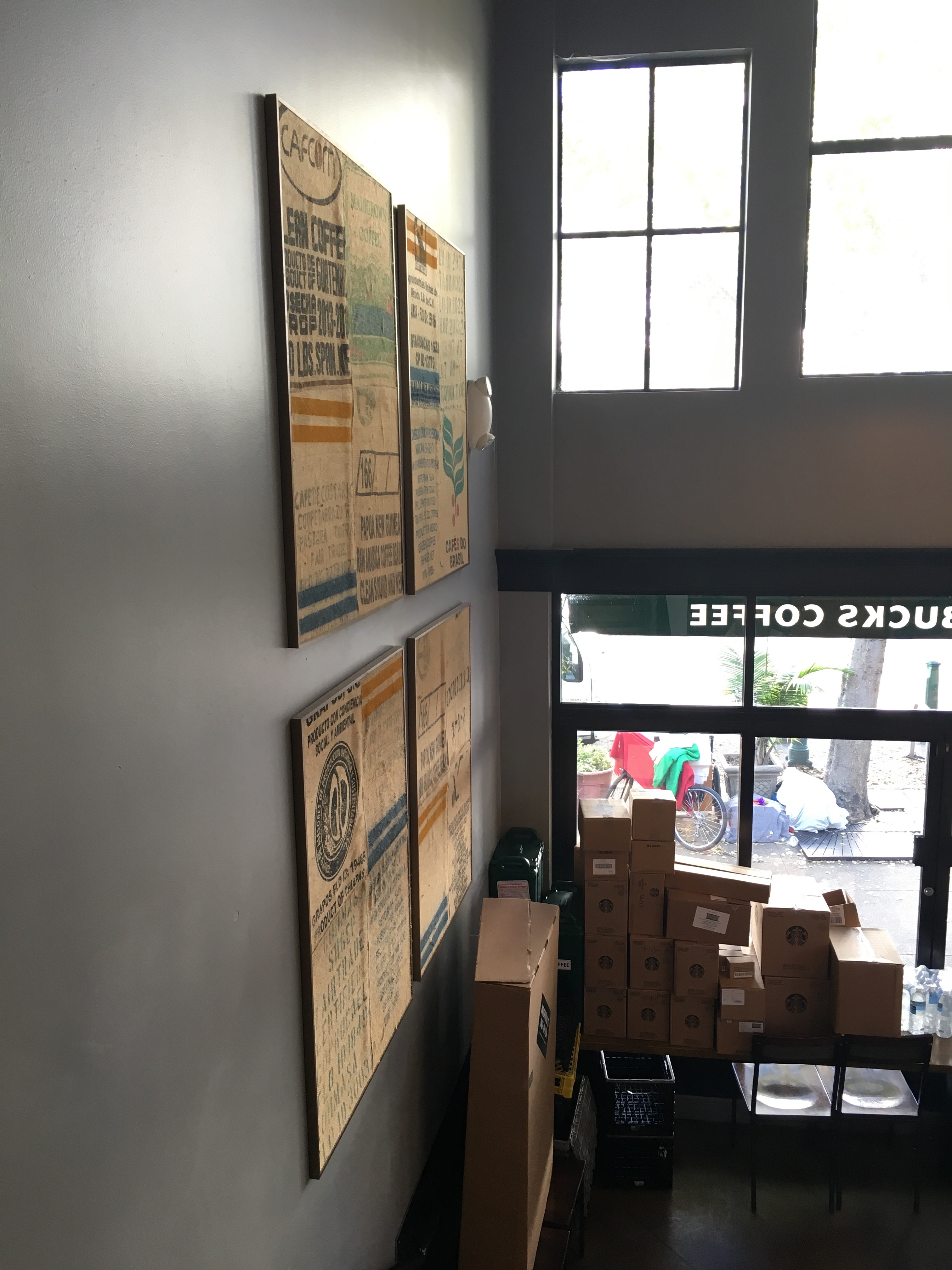
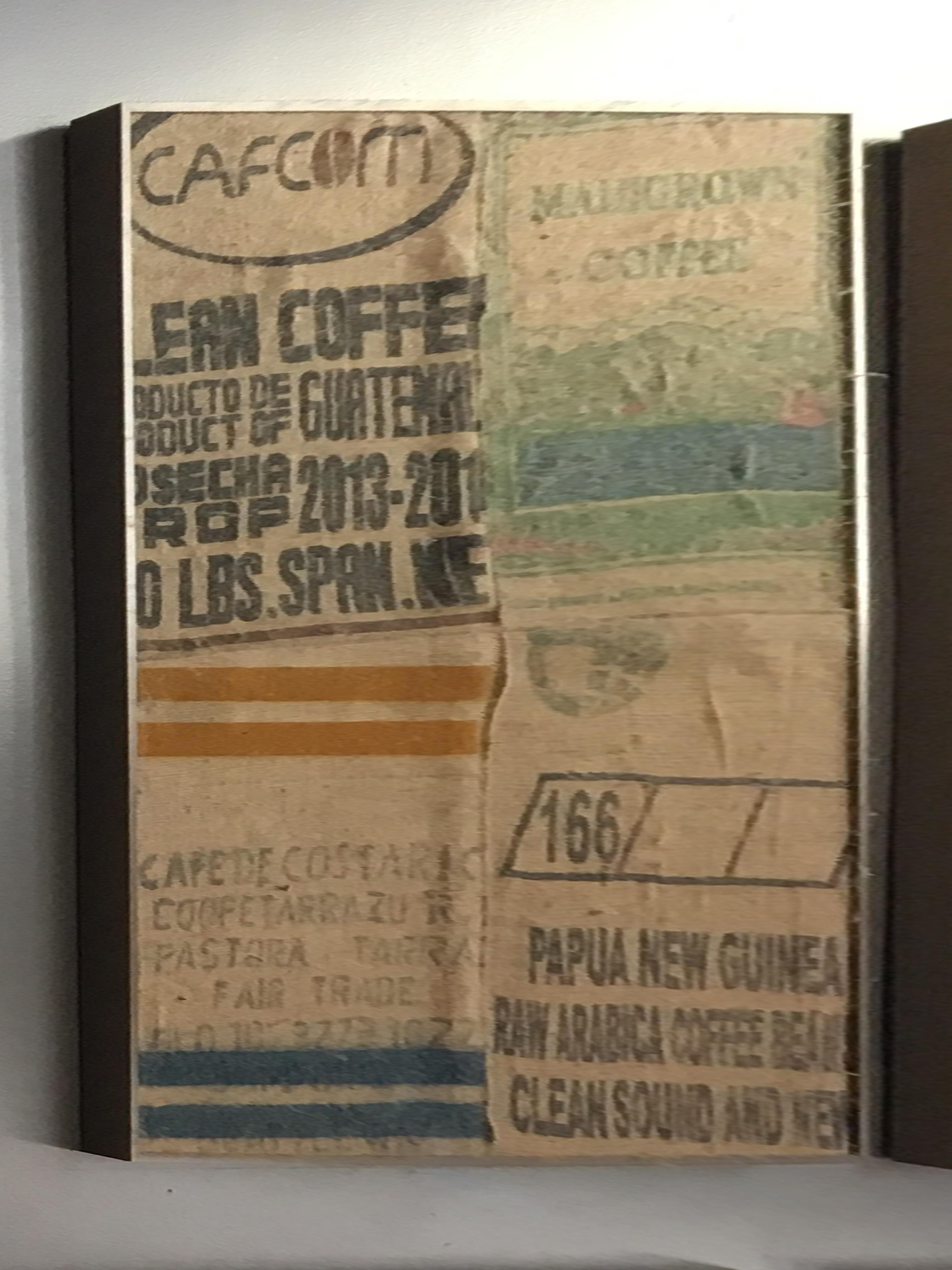
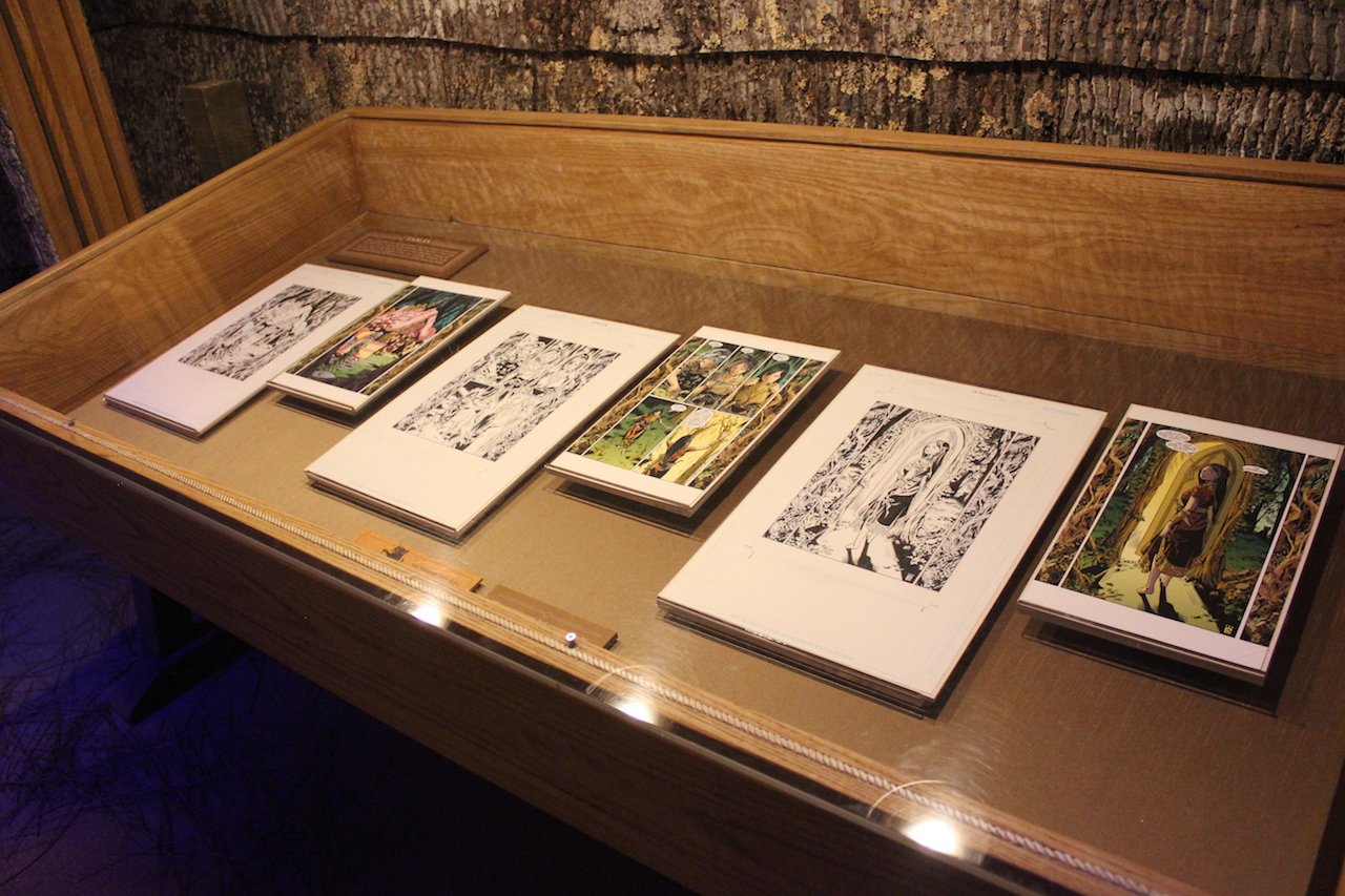
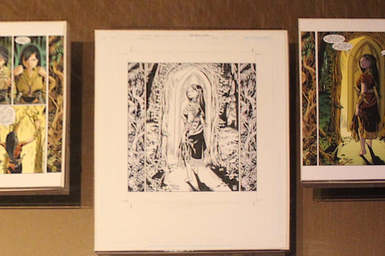
To rectify an image with some planar surfaces, I pick a set of points on the image then define another set of corresponding points by hand, then calculate the homography and warp the image so that the plane is frontal-parallel.
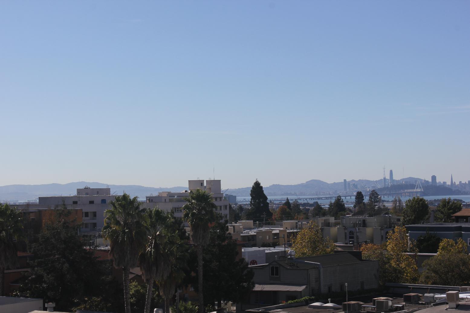
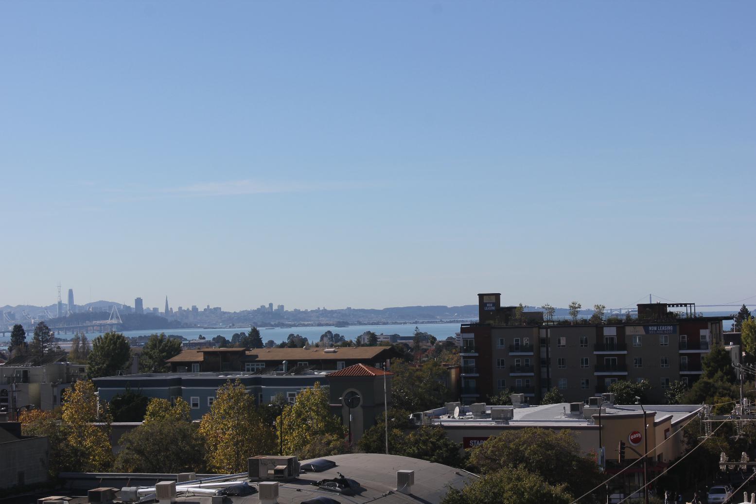
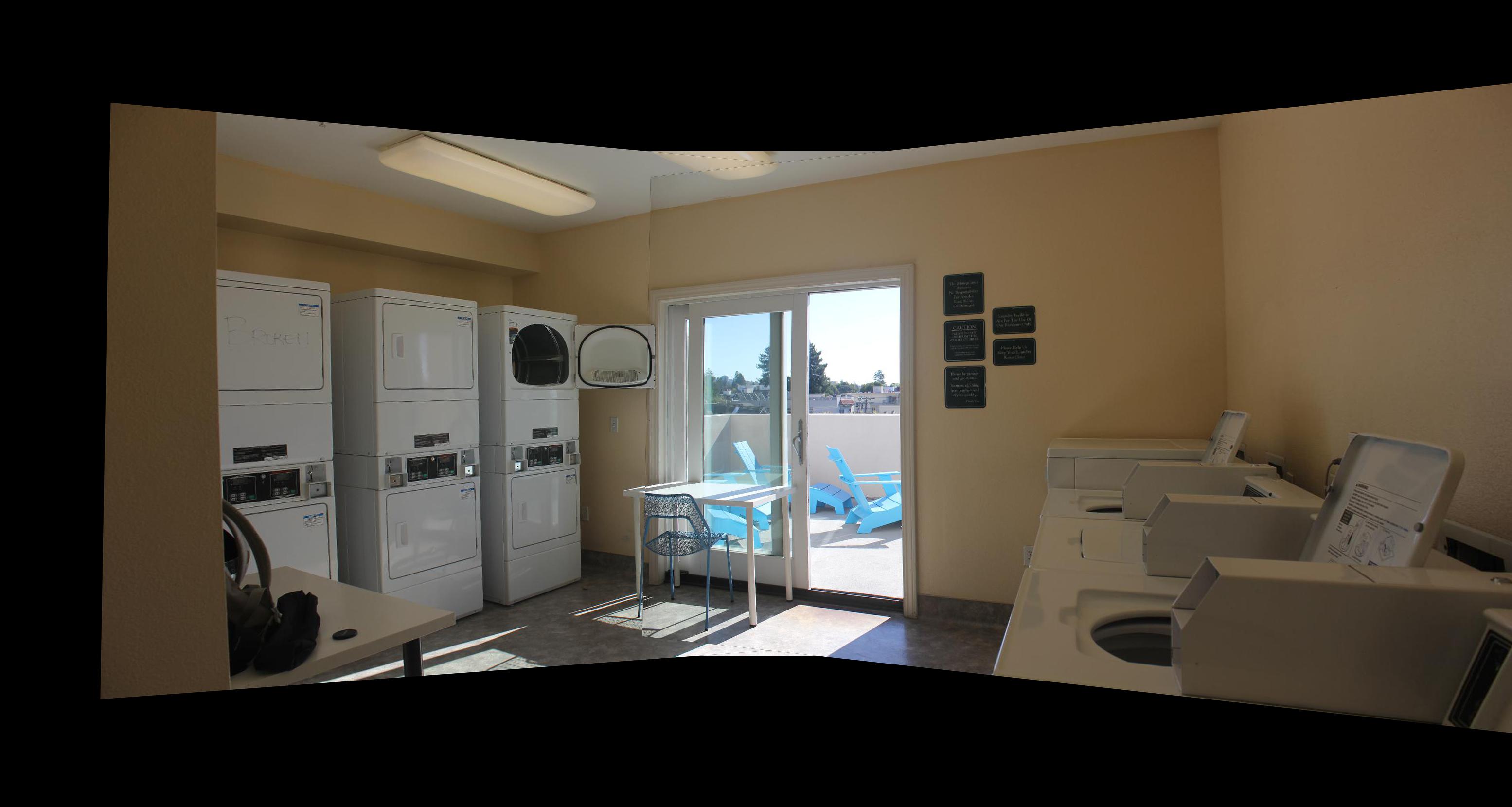
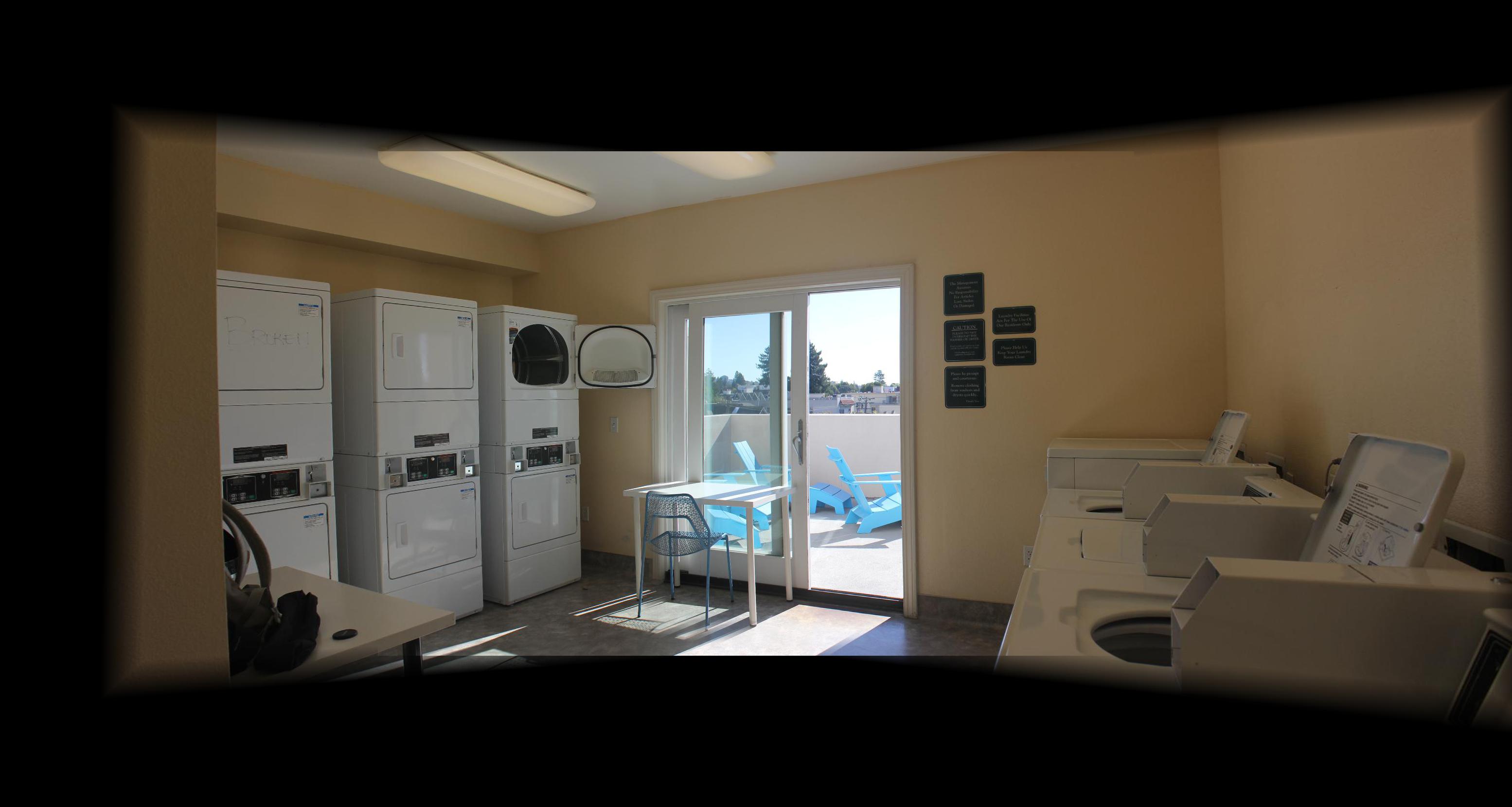
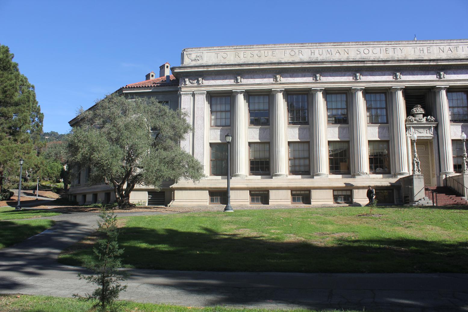
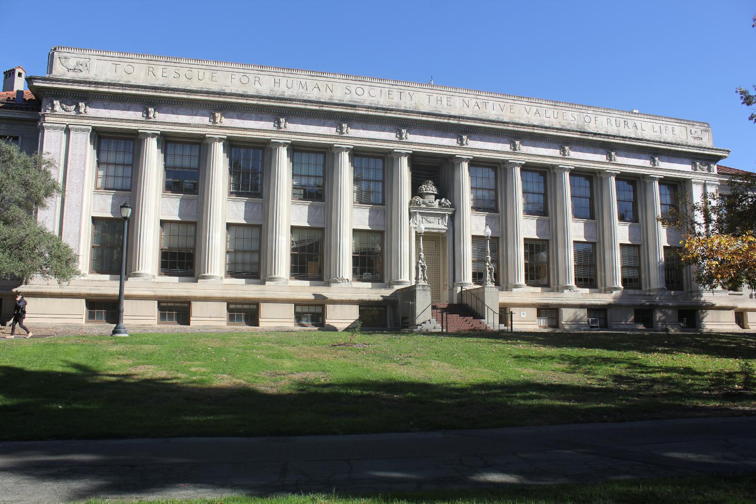
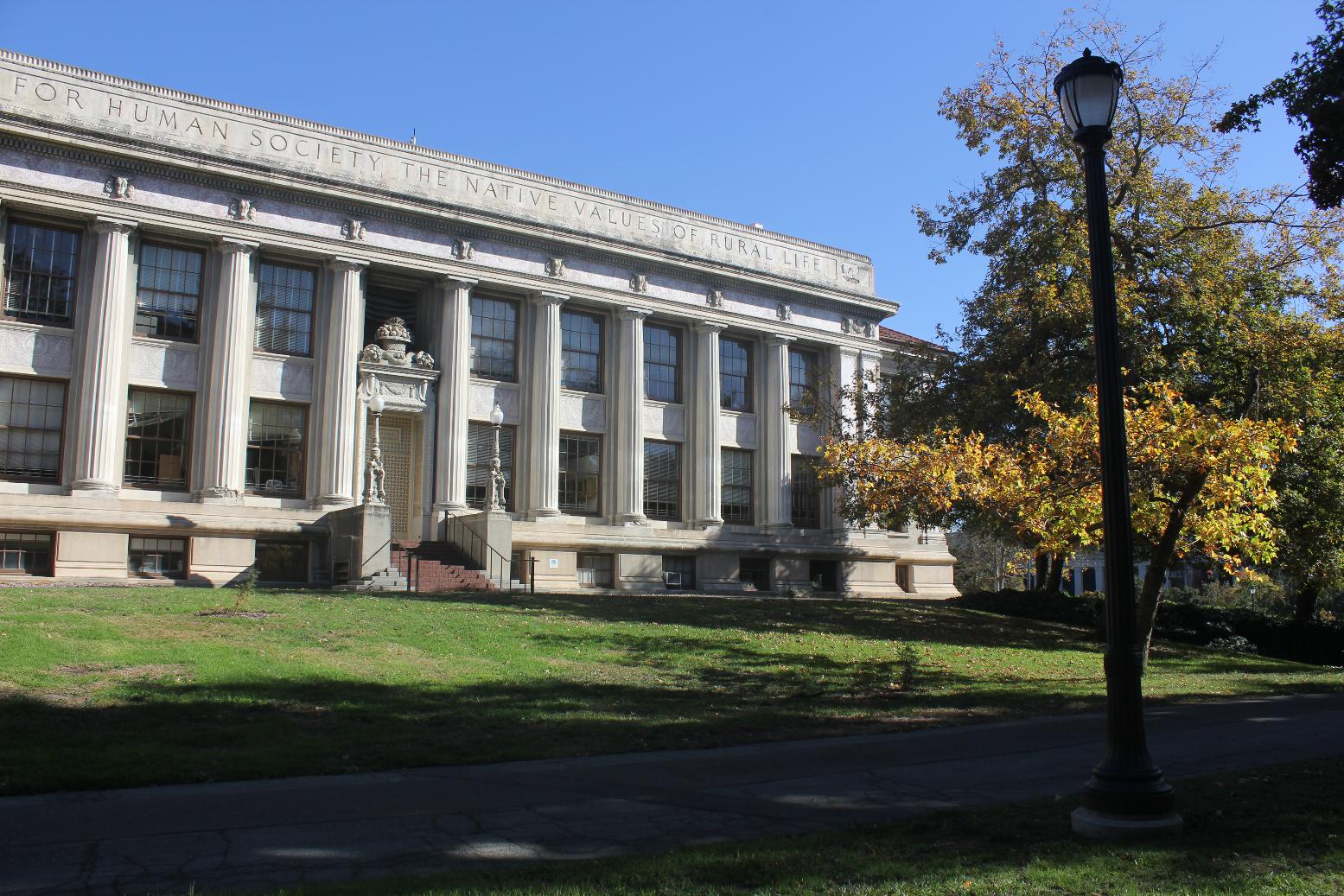
To obtain images to create image mosaics, I took a few sets of photos of difference scenes using a tripod and only changing the view direction. For each set of images, I choose the photo in the center and warp the other images onto its projection one by one. Since I use inversed warping with interpolation to warp my images, I pad each image to the estimated size of the mosaic with black. For blending the results, I also created corresponding masks and warped the masks with the same homography, then I blend together each warped image and the previous result to update the mosaic. Because corresponding points are picked by hand and the brightness of each image varies, just pasting the masked images causes noticeble seams. Therefore, I alternatively blended the images using an alpha channel. The alpha channel I create is basically a mask with value 1 at the center region, and at the edges, the values decrease linearly to 0.
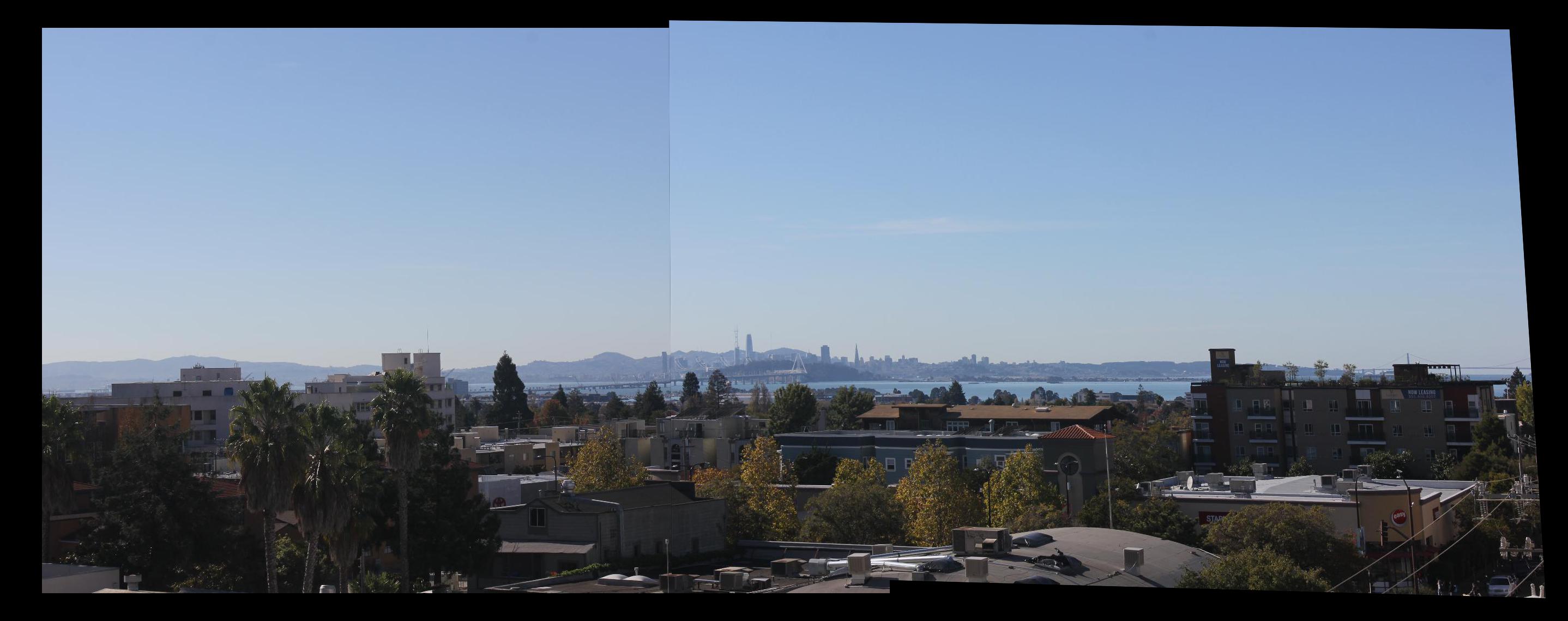
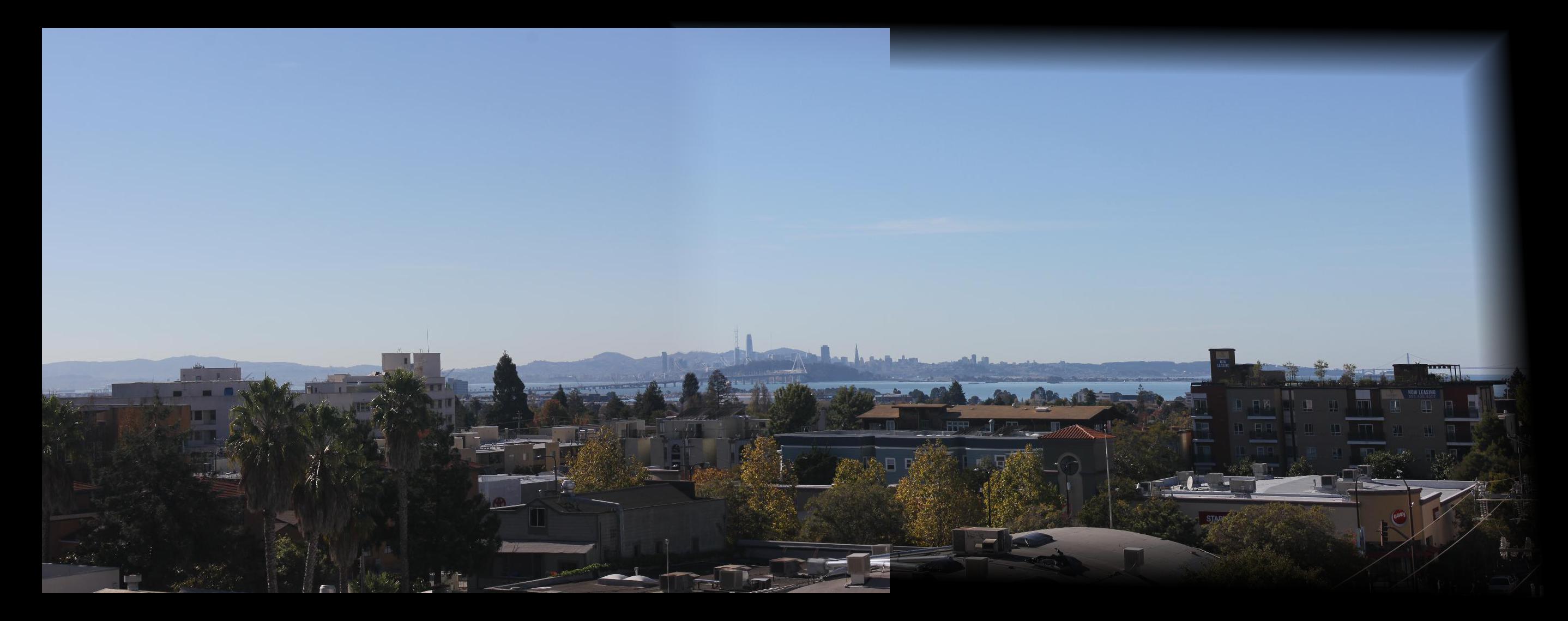
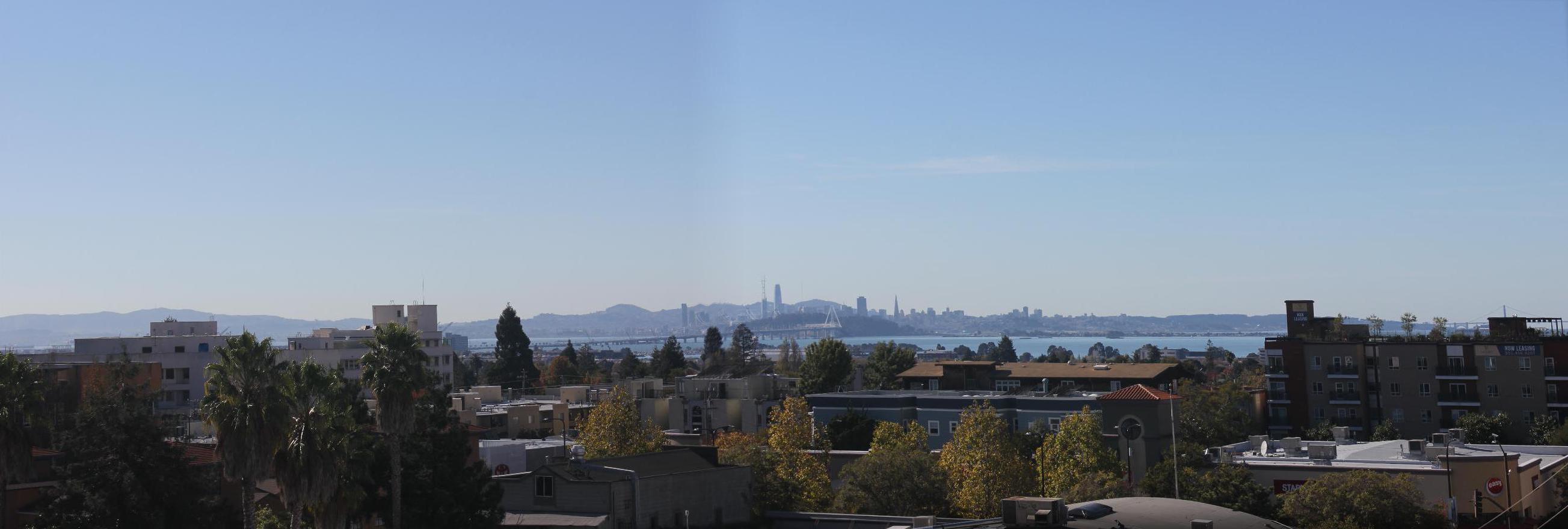
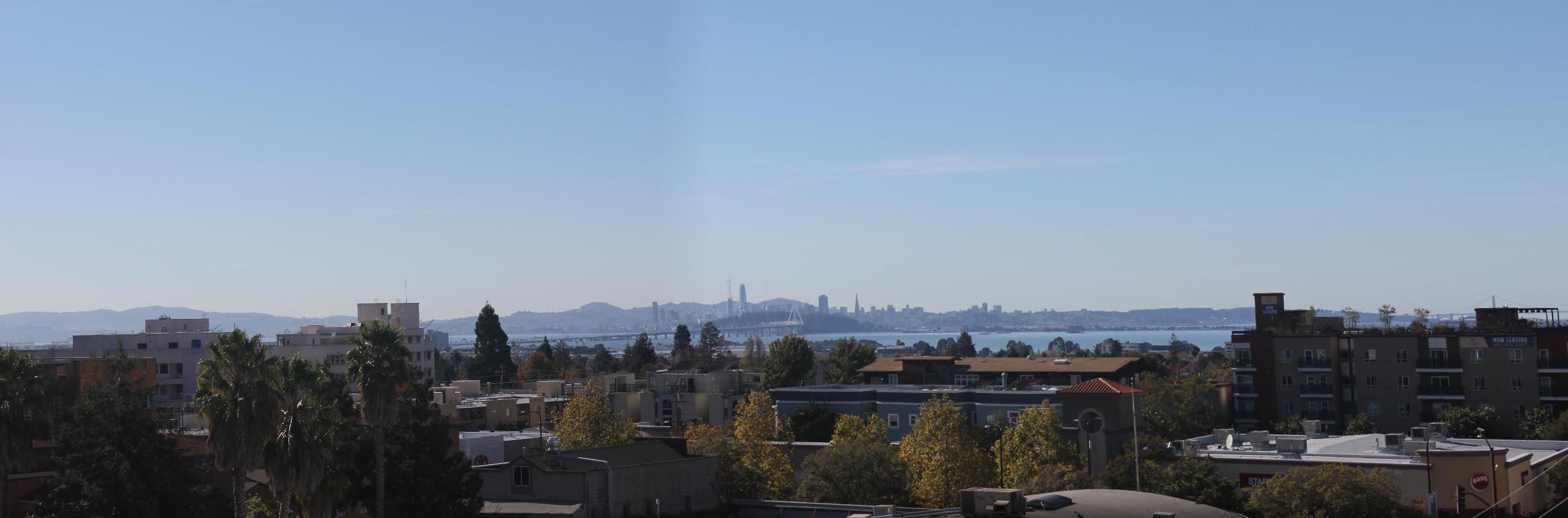
In the mosaic of the bay, because the exposure of the two photos were slightly different, we can see that the color of the sky is not completely uniform.
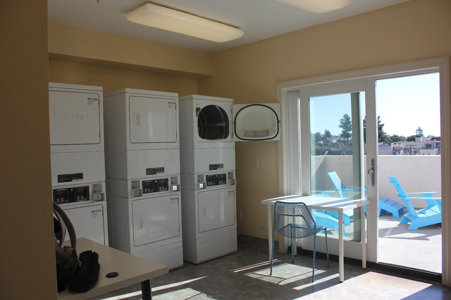
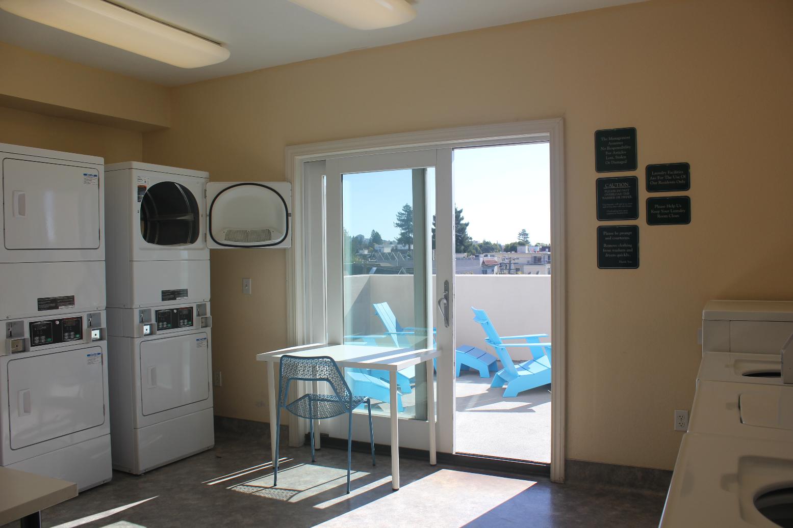
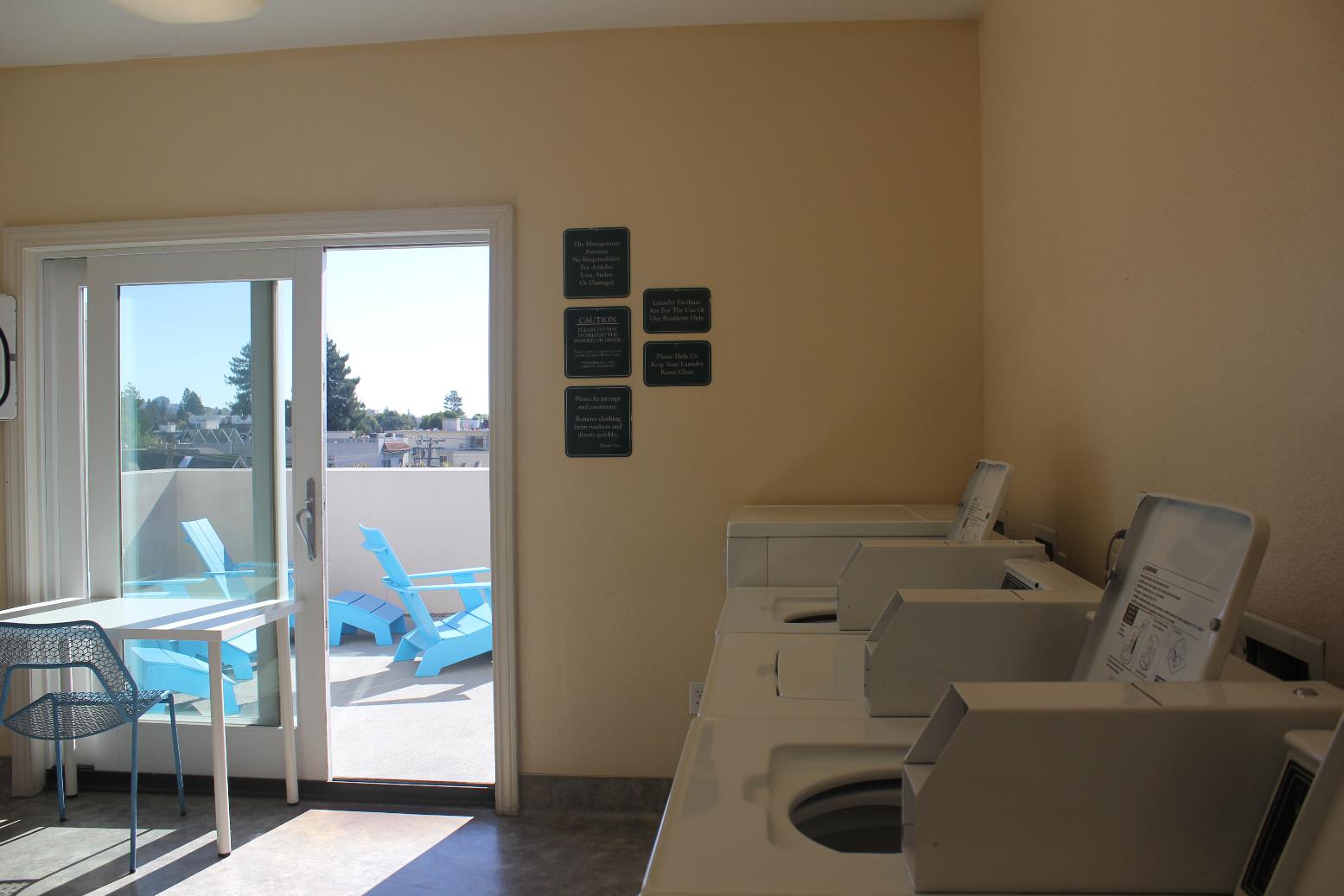
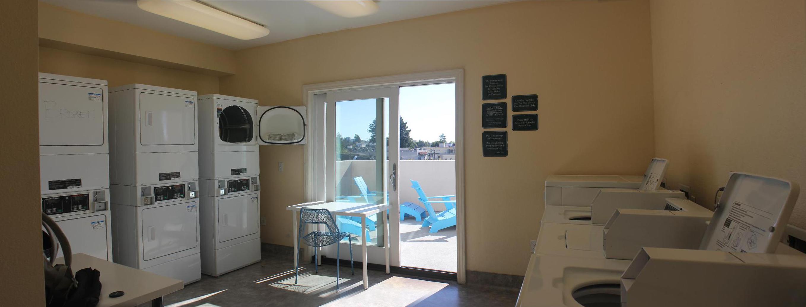
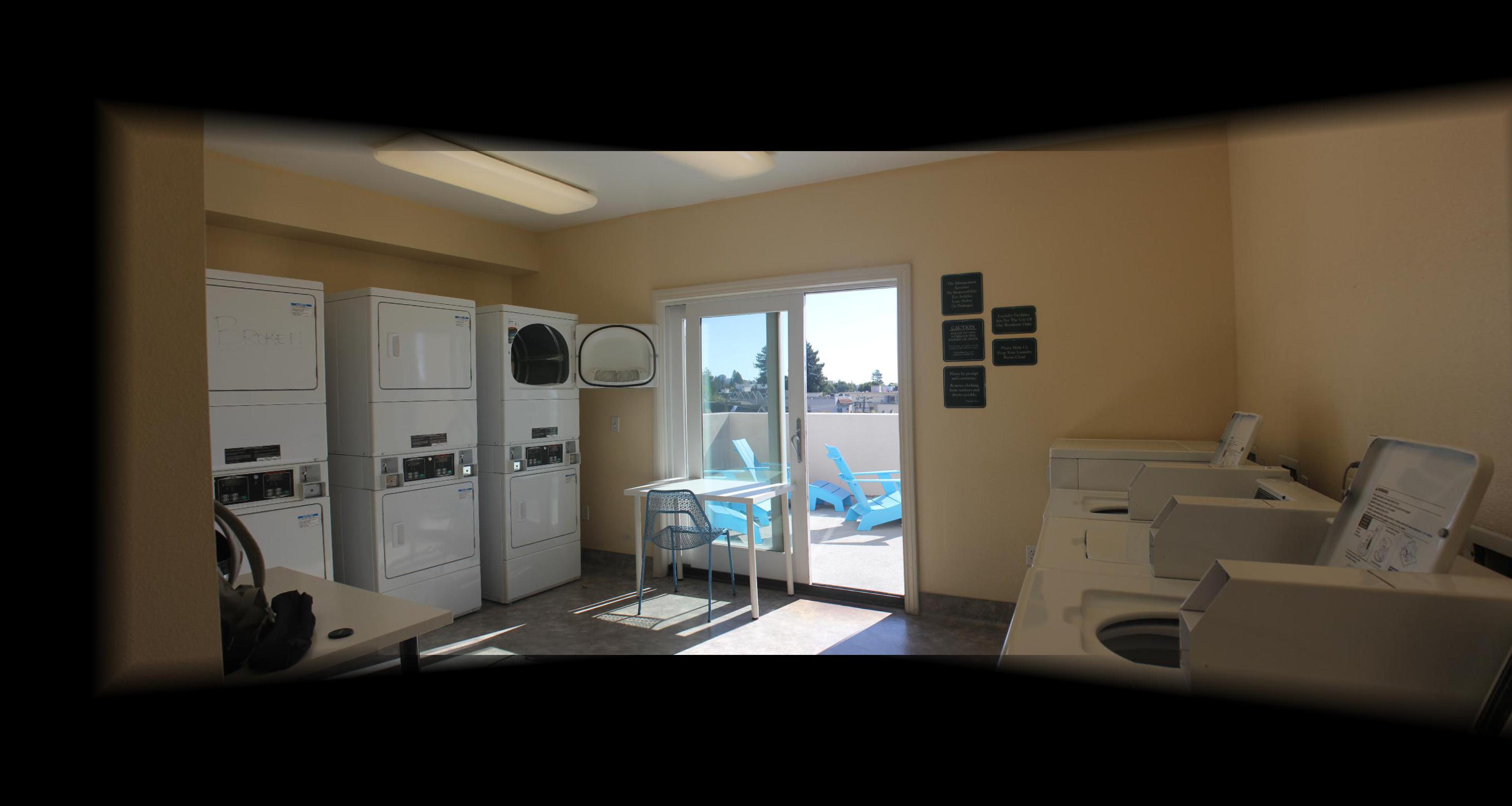
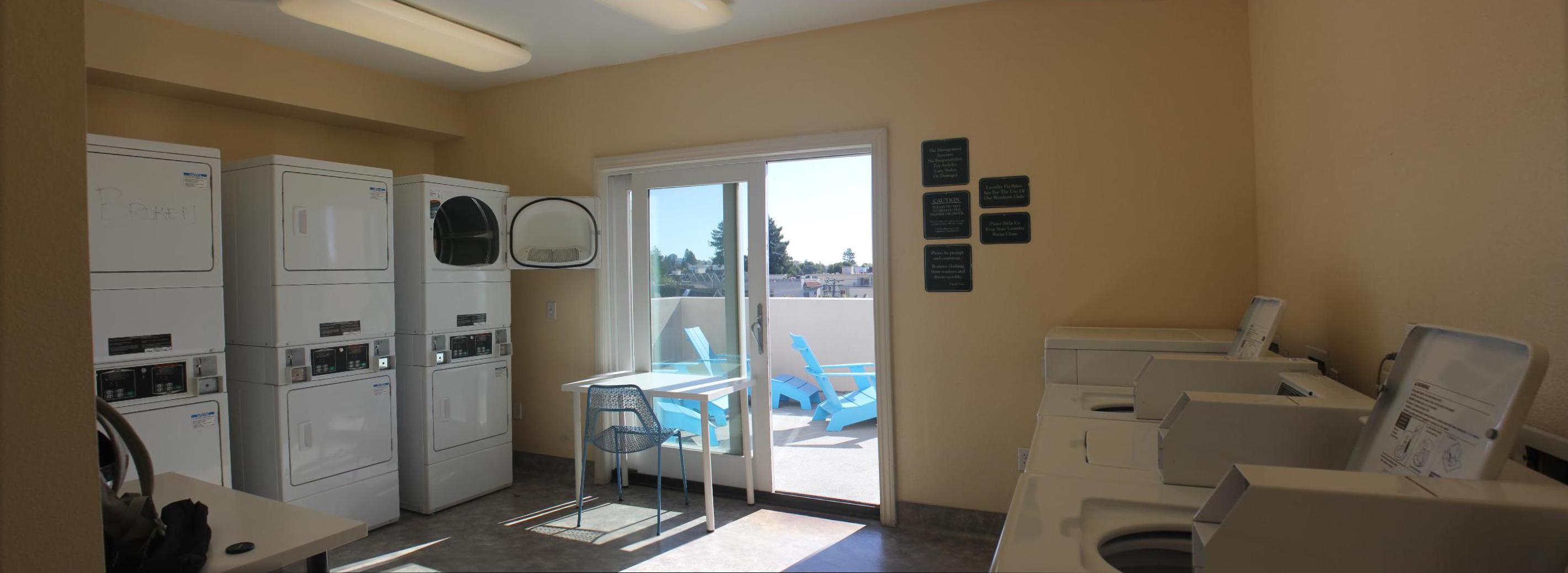
The mosaic of the laundry room turned out very nicely, the brightness in the images were similar enough and the images were warped precisely enough that we don't see obvious stitching seams when using alpha feathering.
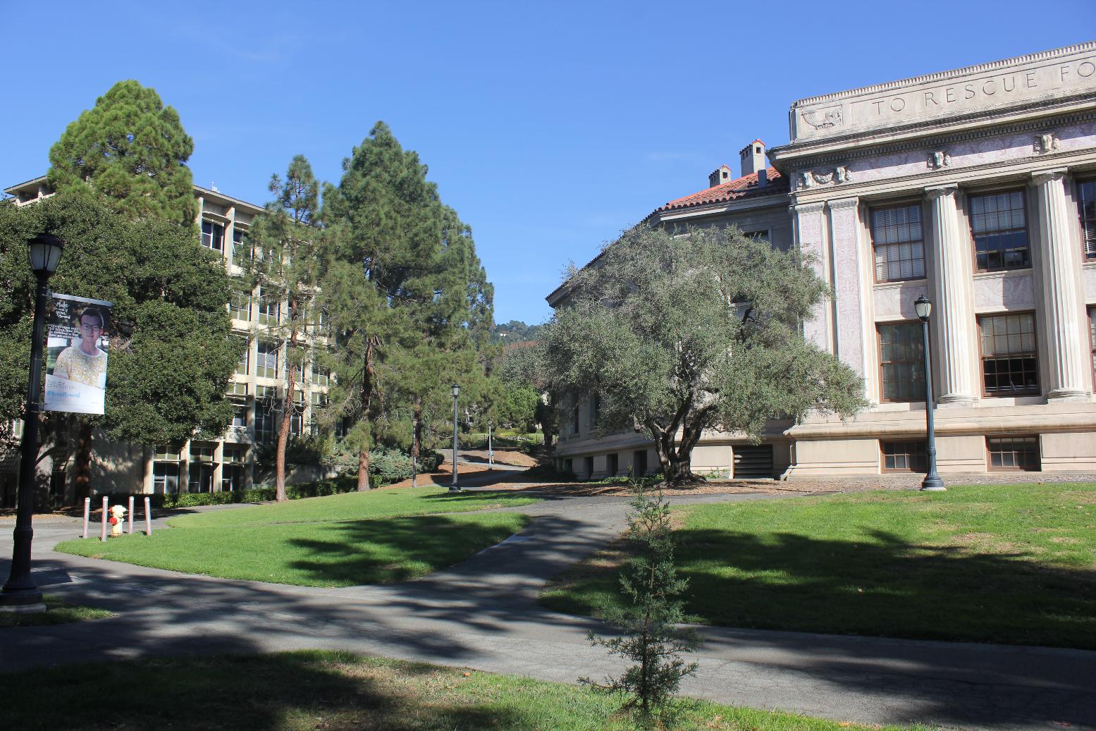
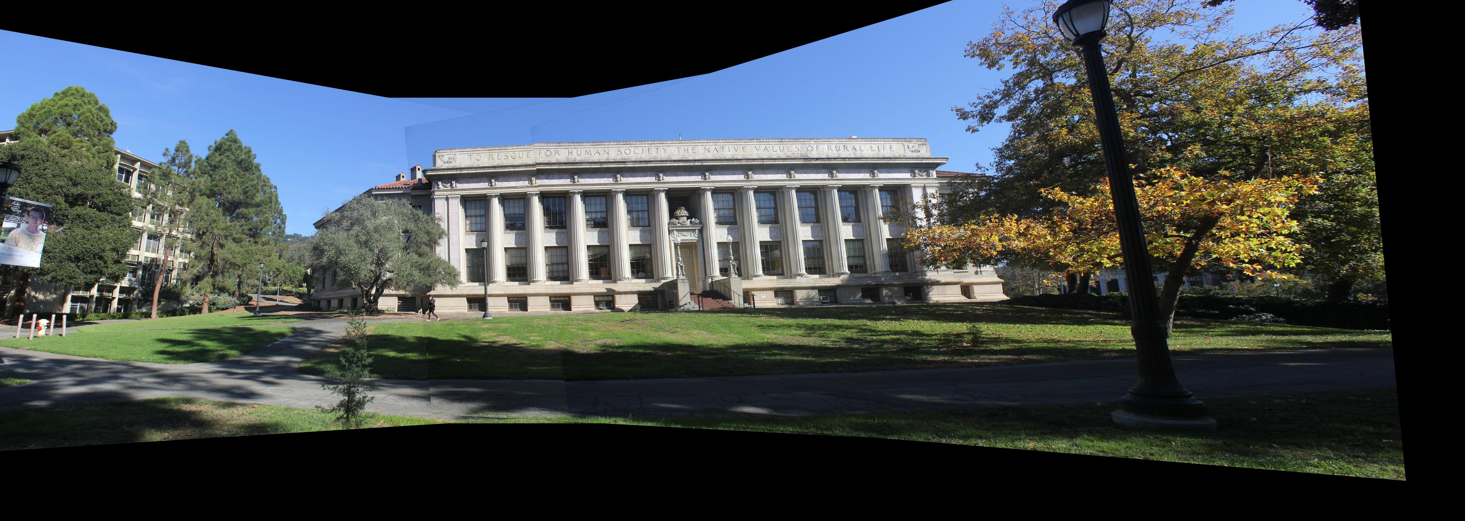
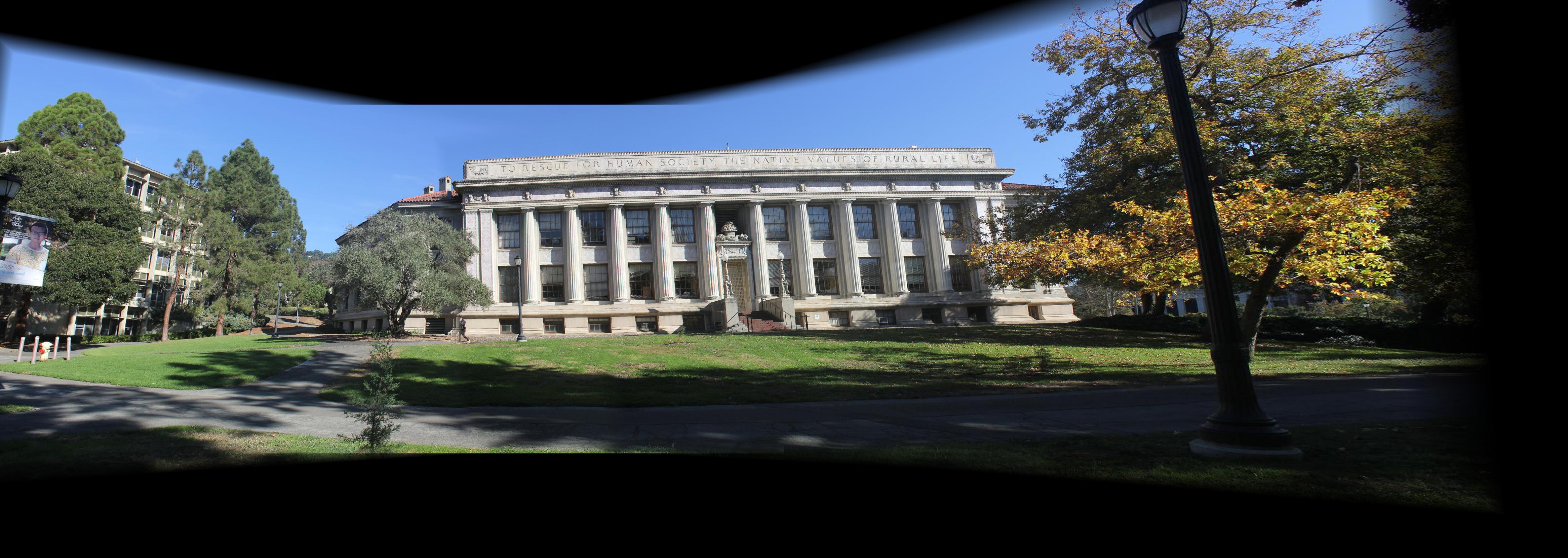
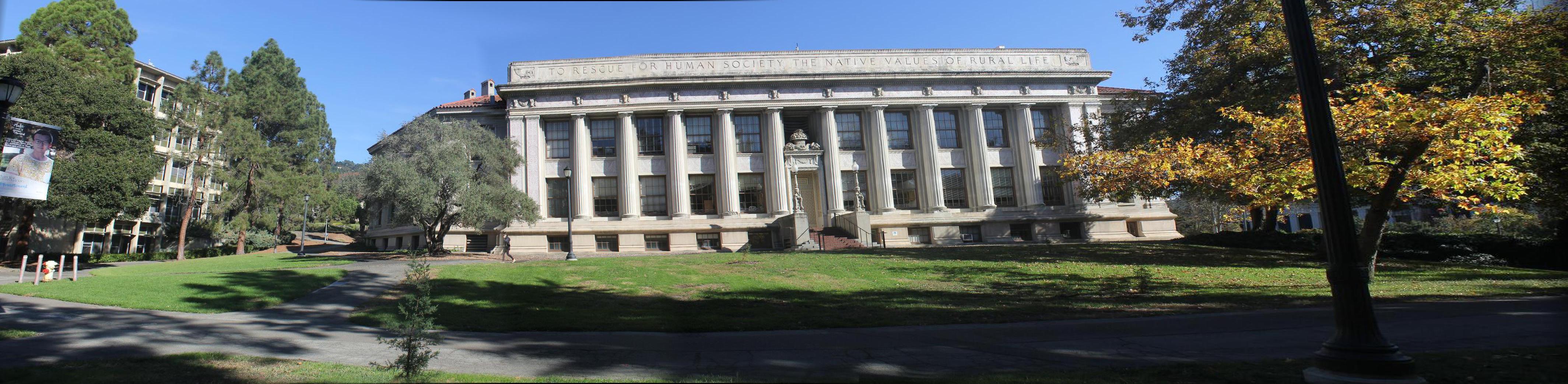
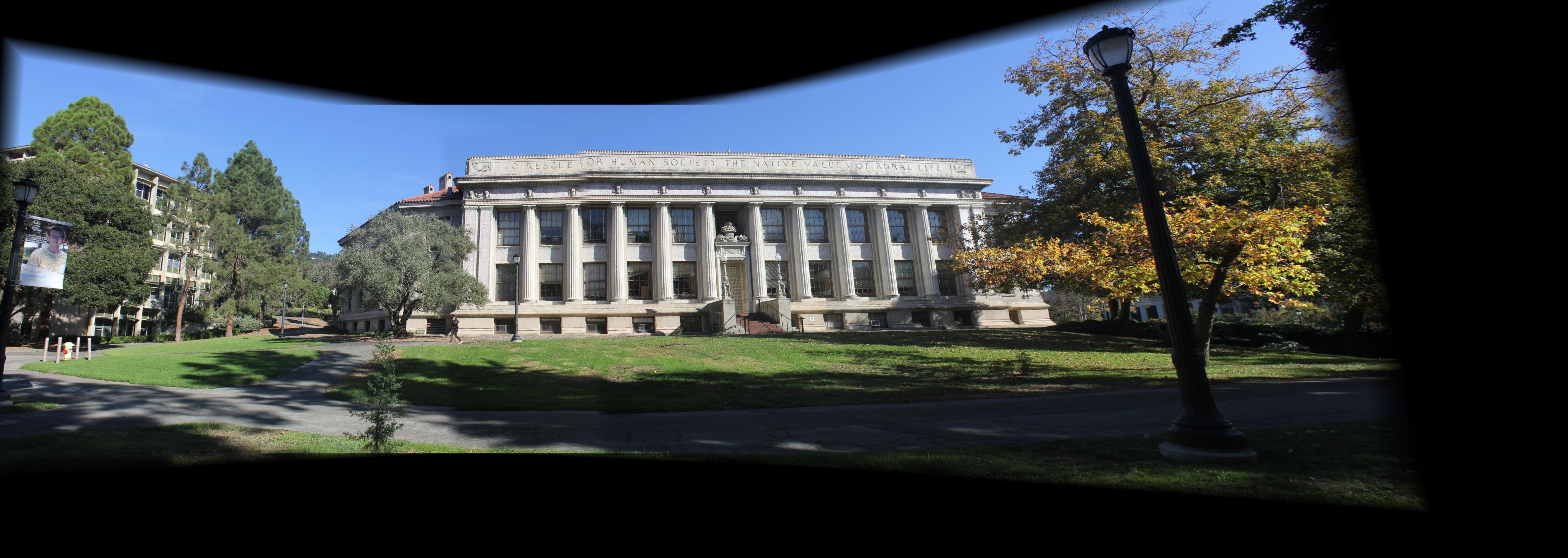
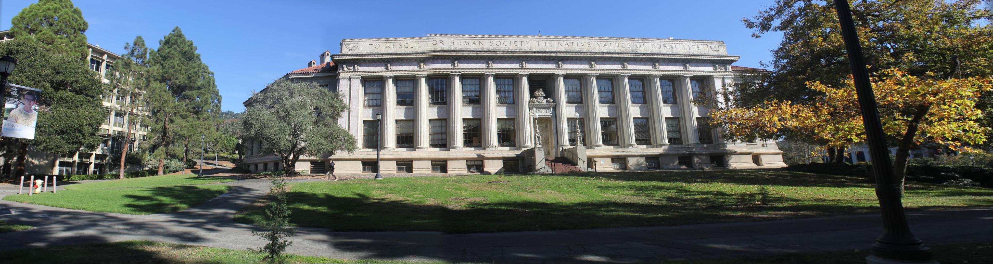
The mosaic of Hilgard Hall is crooked because in the photo I chose to warp other photos to, Hilgard Hall was not forward-facing.
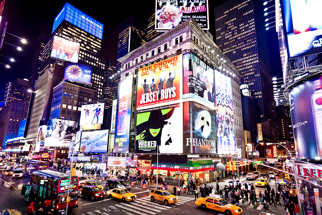
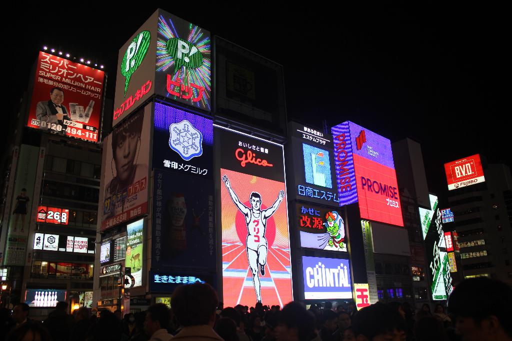
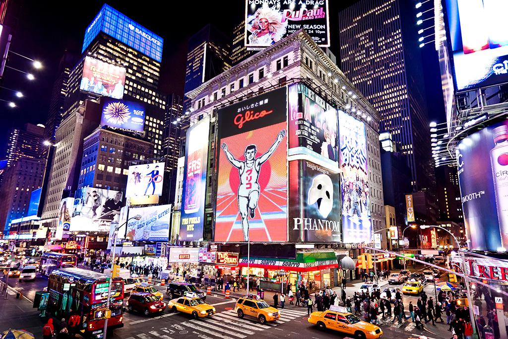
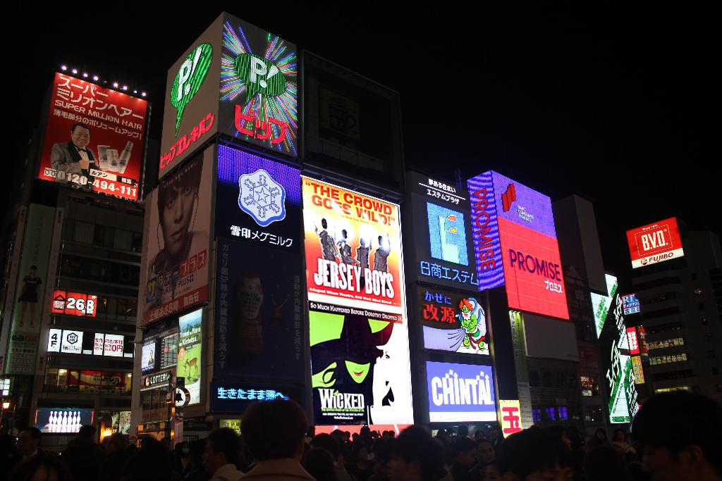
For bells and whistles, I decided to do blending and compositions inspired by the lecture slides. I exchanged the content ofbillboards found in New York and Osaka, Japan.
In the first part, we implemented algorithms to compute homographies given hand defined corresponding points and learned how to create mosaics using homographies. Finding corresponding points by manually clicking on points on an image was not an easy task and the results were not precise and may contain error. In part two of this project, we explore the techiniques used to automatically find matching feature points on a pair of images. Then we use the automatically found feature points to compute homographies and create mosaics.
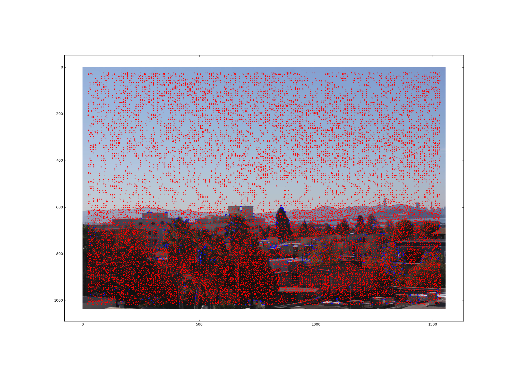
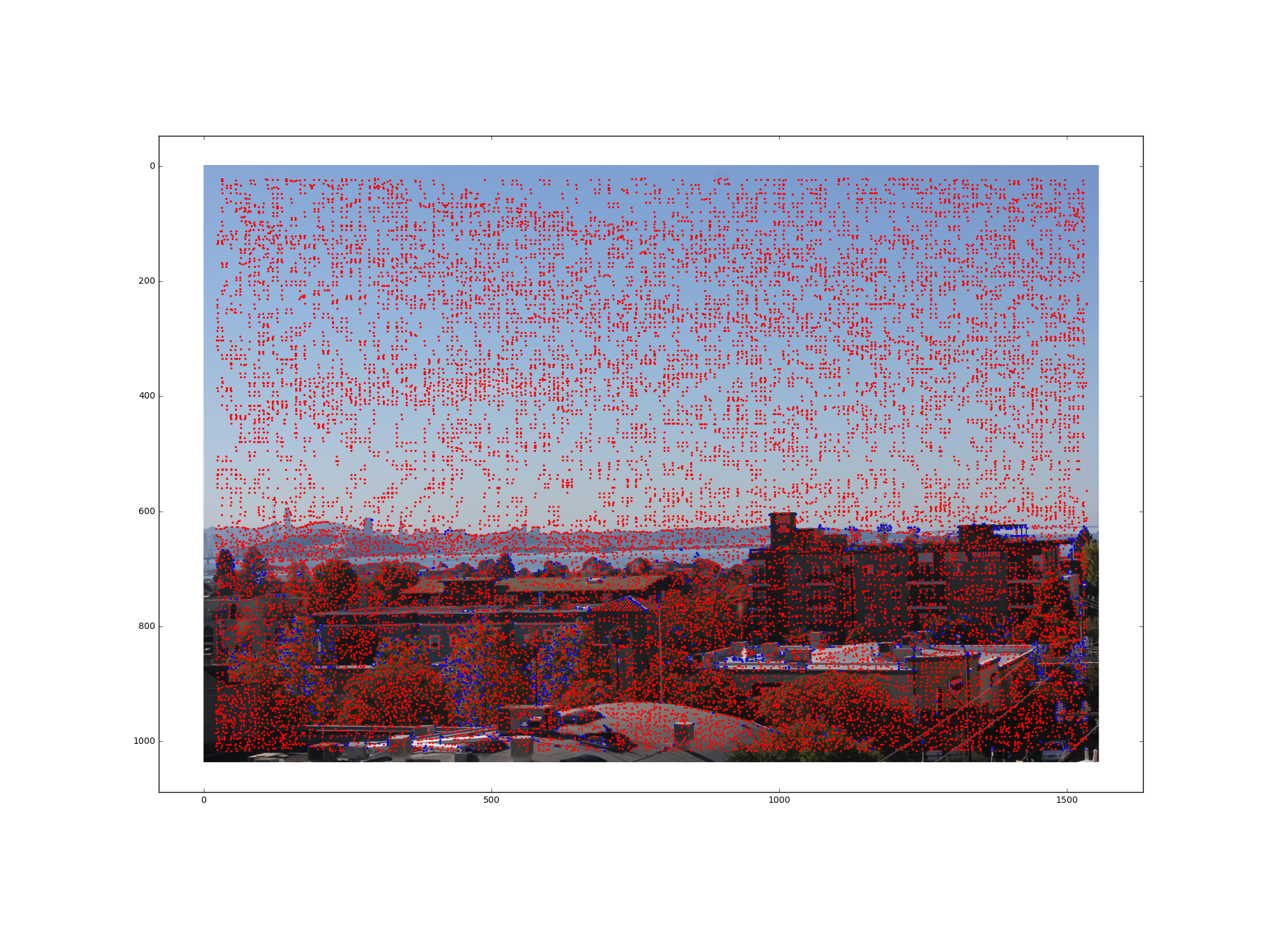
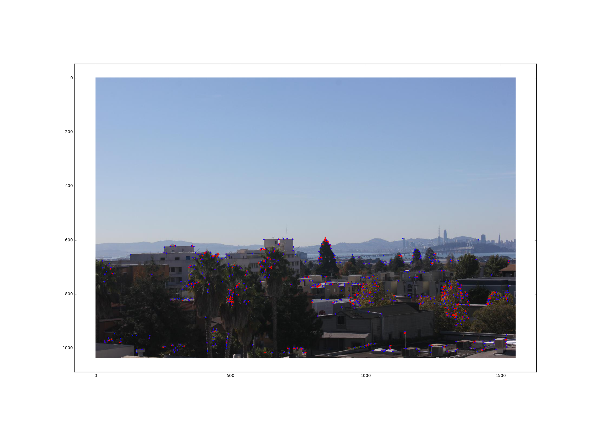
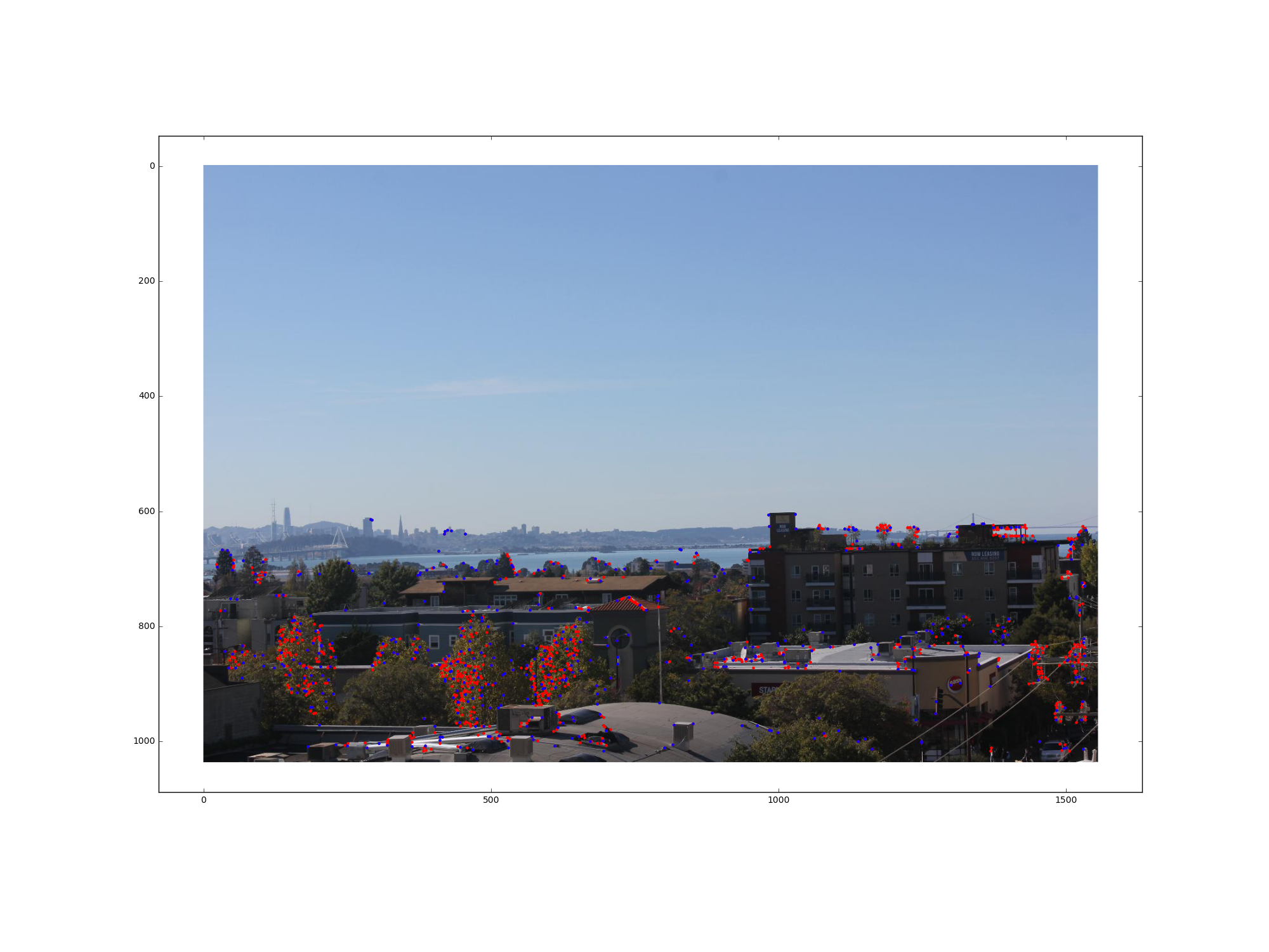
We start with using the Harris Interest Point Detector to find the Harris corners of an image. However, using the sample code provided, we can easily get thousands of points on an image. Therefore, I modified the sample code to use skimage.feature.corner_peaks instead of skimage.feature.peak_local_max. Another way to filter the results is to increase the value of the min_distance parameter of the corner_peaks and peak_local_max functions.
The blue points are the points found by the modified sample code, the red points are the additional points found by the original sample code.
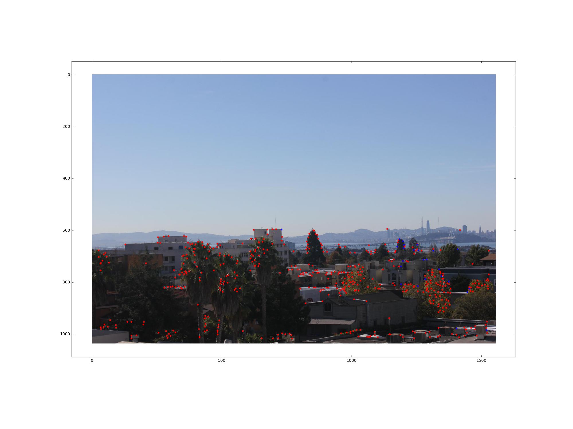
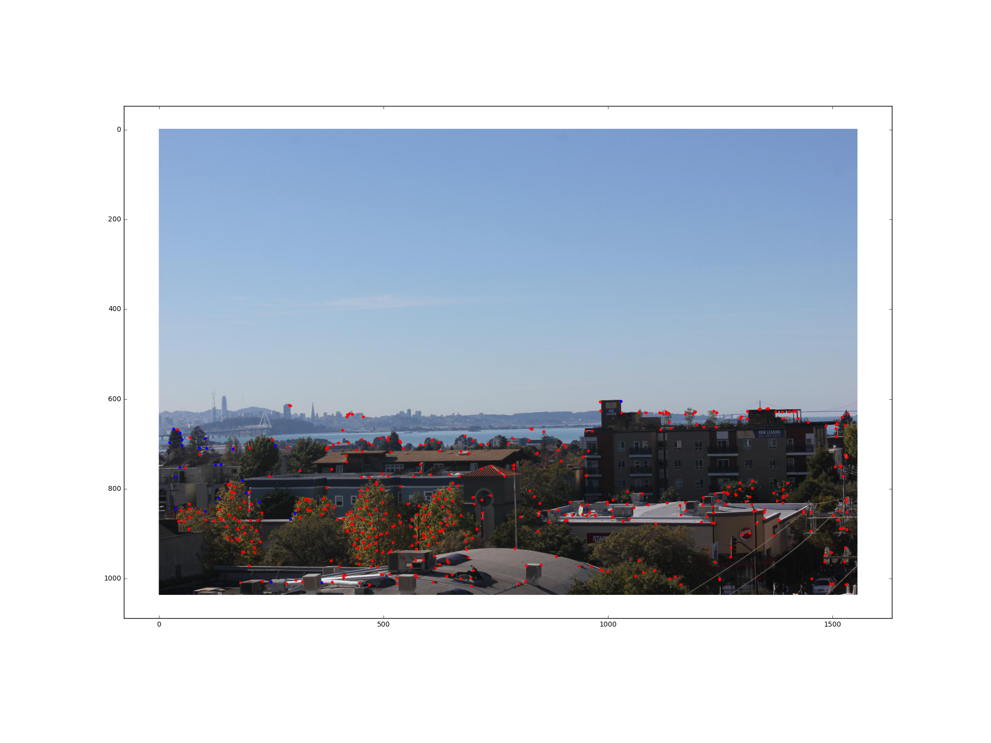
Most of the times, Harris Intereset Point Detection gives us too many points, so we use Adaptive Non-Maximal Suppression to restrict the maximum number of interest points and choose interest points such that they are spatially well distributed over the image. The idea is that we order interest points by their minimum suppression radiuses, which is defined as:  , where x_i is a 2D interest point image location, f(x_i) is the corner strength of x_i, and I is the set of all interest point locations. As suggested in the paper “Multi-Image Matching using Multi-Scale Oriented Patches” by Brown et al, I set c_robust to 0.9 and restrict the number of interest points to 500 according to the descending order of r_i.
The blue points are the chosen points after running ANMS, and the red points are the discarded points.
As stated in Brown et al's paper, once we have chosen interest points, we need to extract a description of the local image structure that will support reliable and efficient matching of features across images. The feature descriptors we use in this project are axis-aligned 8x8 patches represented as a 64 dimensional vector that is bias/gain-normalized so that the mean is 0 and the standard deviation is 1. To make patches less sensitive to the exact feature location, we first sample a 40x40 patch and then downsample it to a 8x8 patch.
After we have extracted the feature descriptors, we match feature points using SSD and an outlier rejection procedure based on the noise statistics of correct/incorrect matches. Detailed speaking, for each feature point we want to match, we calculate the SSD of the feature descriptor with every feature descriptor of the other image. Then, we choose the matching feature descriptor that gives the smallest SSD. However, we also need to decide whether the match is an outlier by checking if ratio of the SSD with the best match and the SSD with the second best match is larger than a threshold. Based on the statistics and figures in the paper from Brown et al's paper, I chose 0.4 to be the threshold.
The blue points are the feature matches found, and the red points are the discarded feature points.
For the last step of automatically finding corresponding points, we use RANSAC to compute a robust homography estimate:
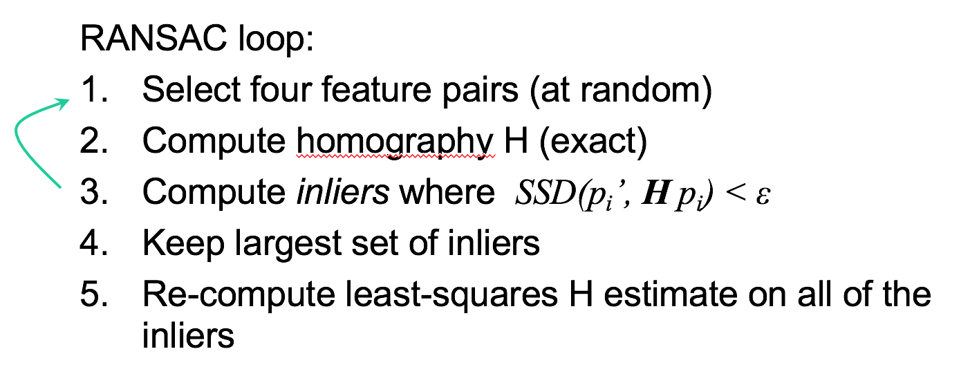 .
.
I chose to run the loop 10,000 times to get the largest set of inliers.
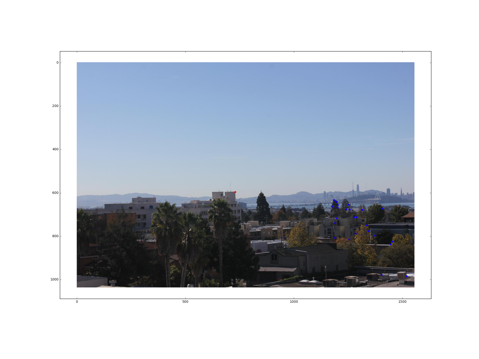
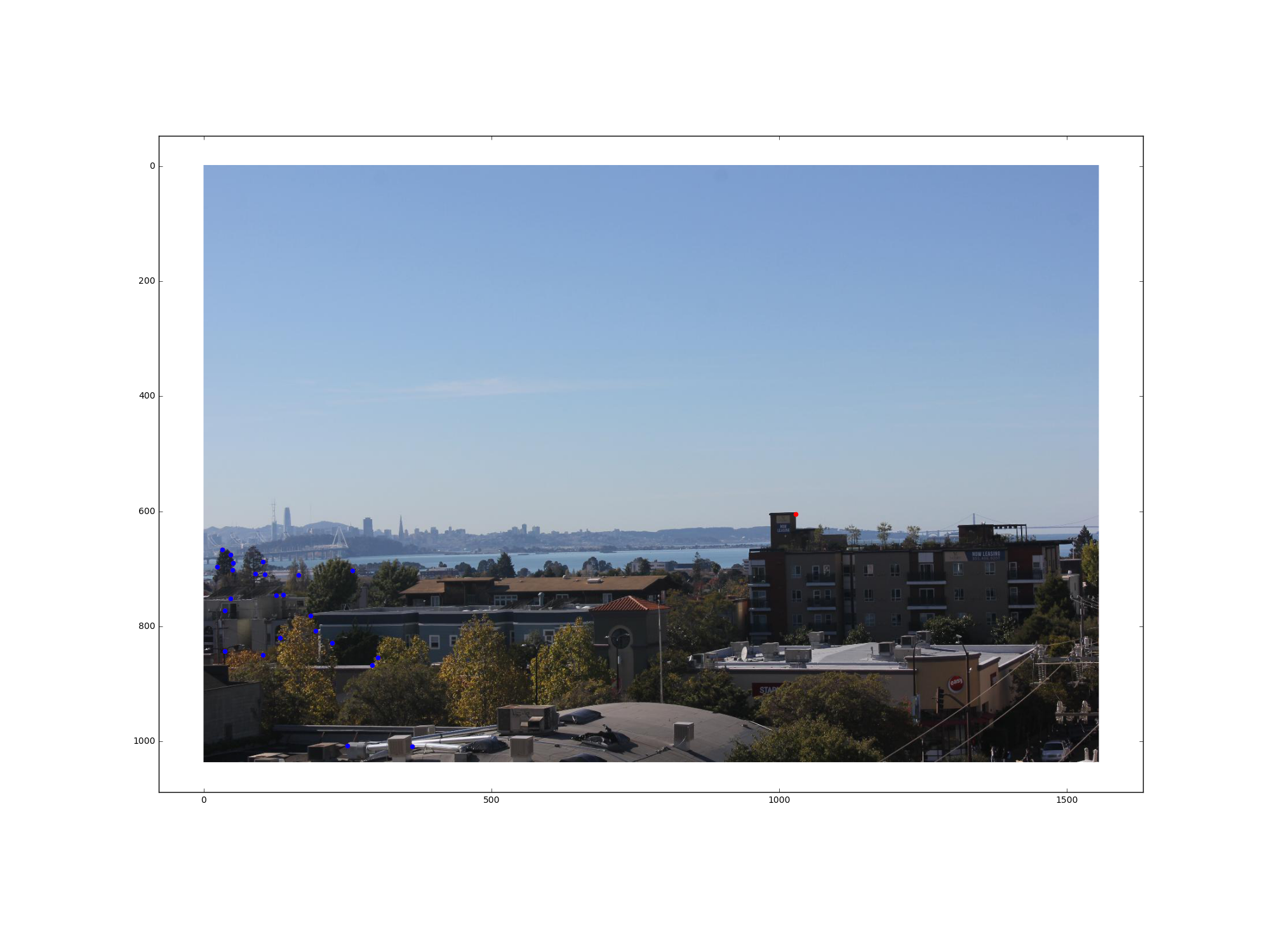
The blue points are the kept points after running RANSAC. You can see that RANSAC got rid of a pair of outliers, shown as a red point on each image.
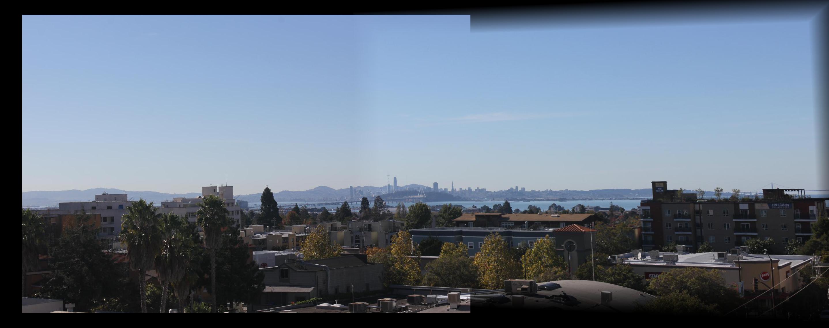
Now that we can automatically generate a set of matching features and compute robust homography estimates, we can use warping and blending techinques developed in part 1 to create mosaics and compare how the results come out.
The mosaic for Hilgard Hall displays an obvious difference between using hand defined and automatic generated corresponding points. When I hand defined corresponding points, I deliberately chose some points very close to the edges so that I could have a better seam. Although the mosaic created using automatic generated corresponding points has a more obvious seam, which is probably due to the radial distortion of flawed lens, the overall mosaic is not as distorted and looks more natural than the mosaic created using hand defined points.
This project was really fun because we got to make mosaics using our own photos and we also used a lot of techniques we have learned from past projects, such as image warping and blending. For this project, it turned out that getting the image blending to look right took the most amount of time, mostly because it was difficult to use more complicated blending methods like laplacion blending as it was hard to deal with the black padding around the images, which we don't want to blend. It was also not trivial to create masks with alpha feathering for the blending. If I had more time, I would definitely want to try to make laplacian blending work. Also, although ANMS turned out the be the slowest to run in part 2, mostly because it took a long time to sort a large array, automatically finding corresponding points was still much, much more efficient than hand defining points. So this project really made me appreciate the people who came up with algorithms to automate processes that may take a long time to be done manually.