In this project, we select corresponding features between pictures that contain the same features and then calculate a homography based on point correspondences. We use the homography to then warp images into the same image space so that they can be superimposed and blended to stitch them together into a larger continuous image. We model our homographies as projective transformations with eight degrees of freedom (the matrix has eight unknowns). Therfore with at least four correspondences we can construct a system of equations to estimate a homography.
Shoot the Pictures
I took pictures with my glorious Pixel 2.
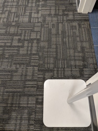
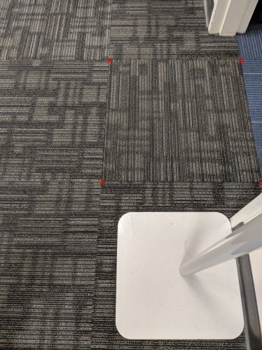
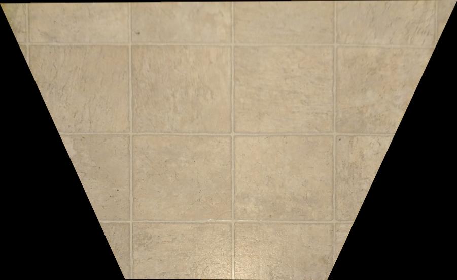
Soda 277 Floor
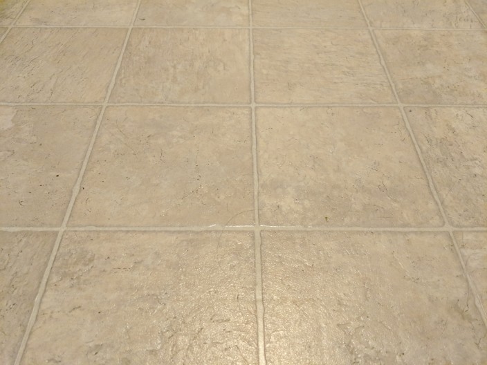
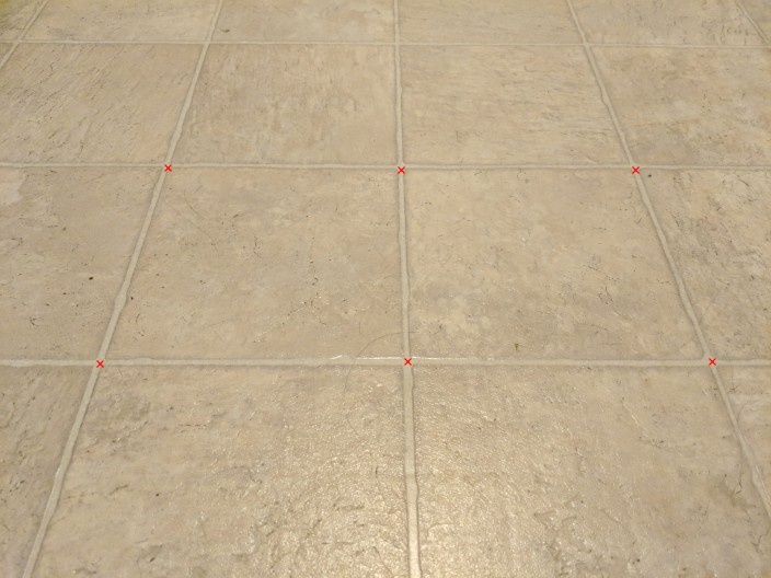
Kitchen Floor
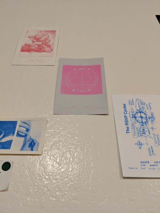
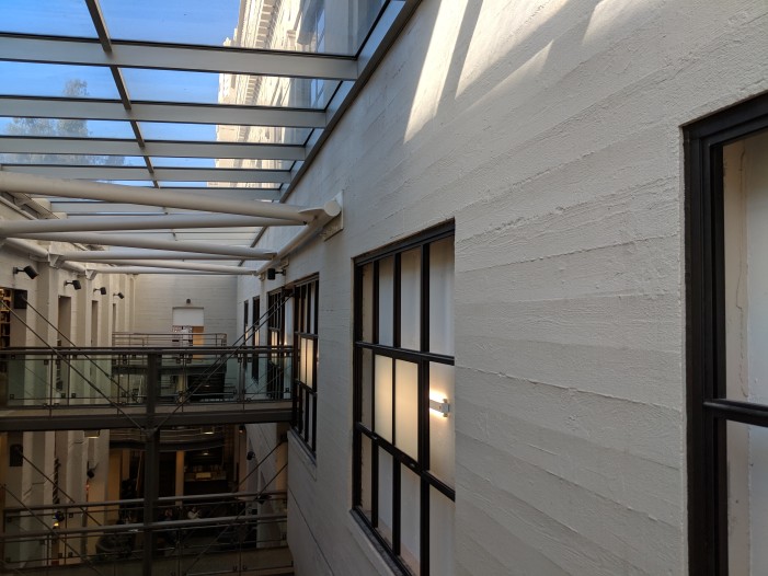
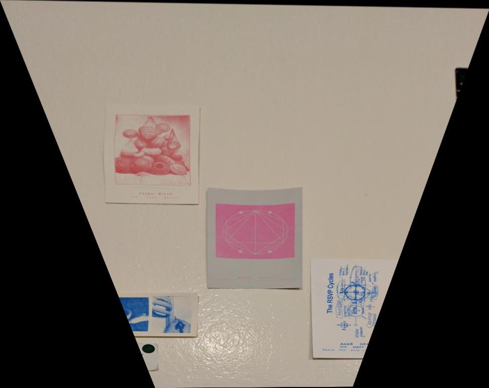
Wall Above My Desk
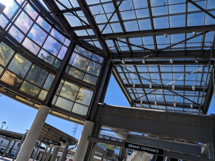
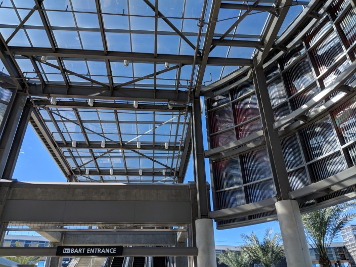
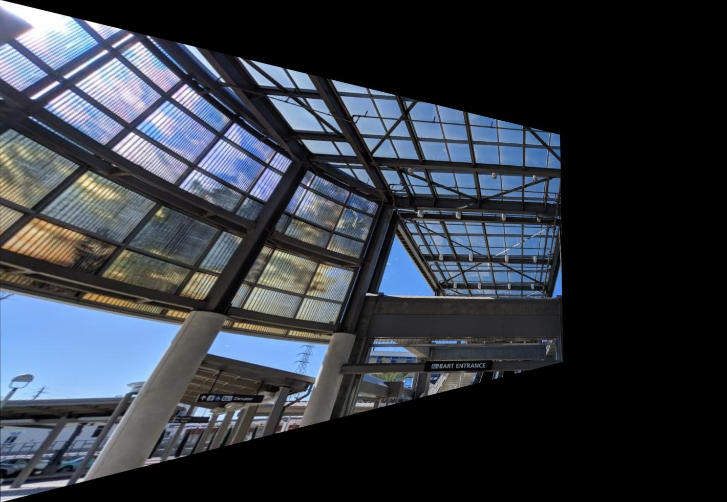
Warm Springs/South Fremont BART Entrance Left
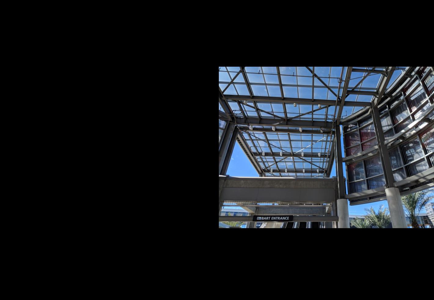
Warm Springs/South Fremont BART Entrance Center
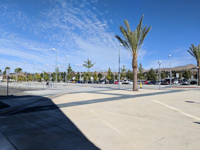
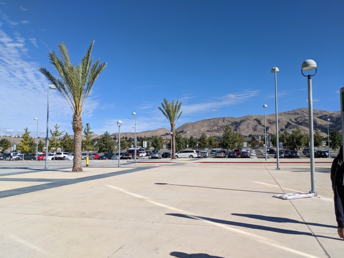
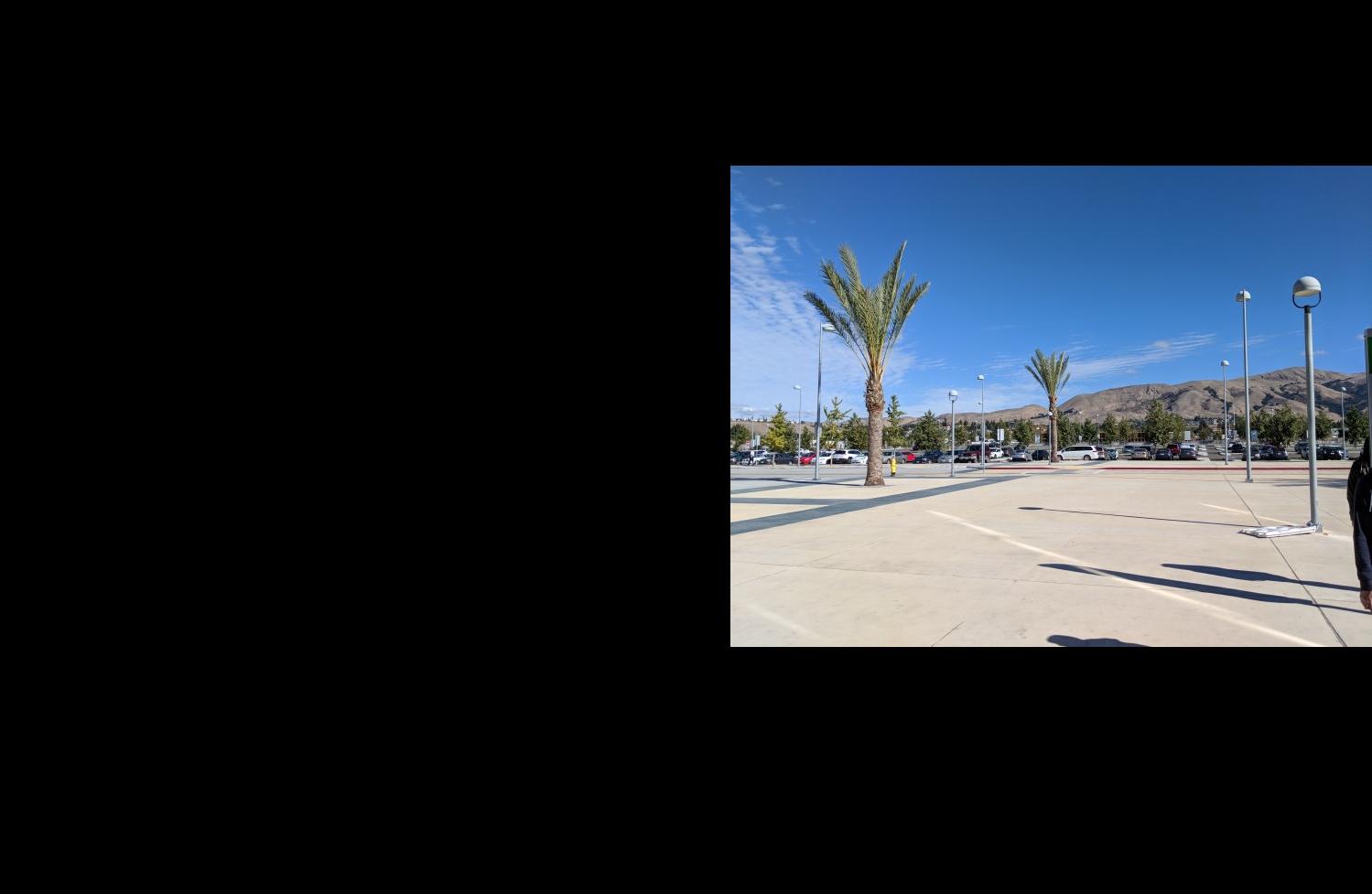
Warm Springs/South Fremont BART Plaza Center
Warm Springs/South Fremont BART Plaza Right
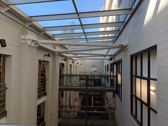
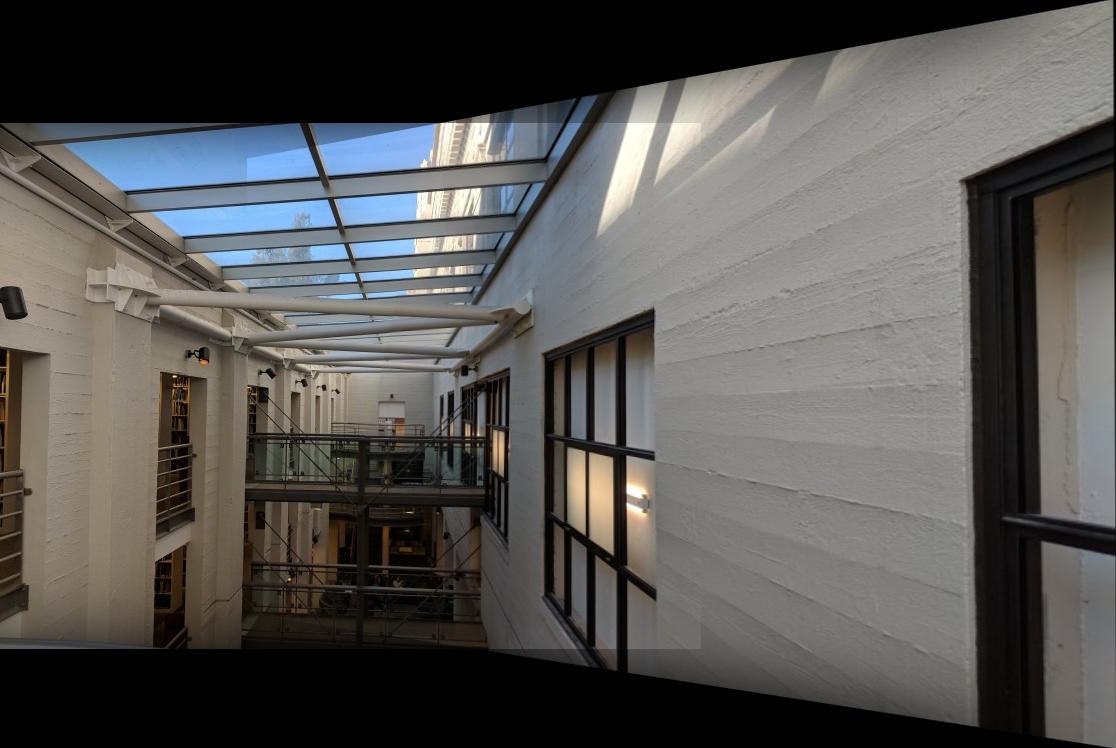
Marian Koshland Bioscience & Natural Resources Library Left
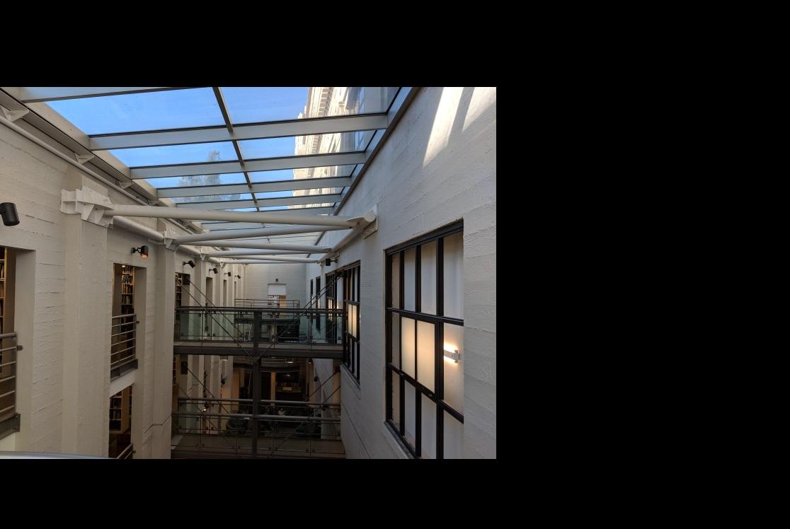
Marian Koshland Bioscience & Natural Resources Library Center
Image Rectification
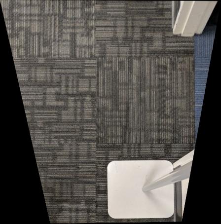
First, I tested my homography computation and warping by checking that I could correctly retify objects in images. I took pictures of rectangular objects at slanted angles and then picked flat correspondences (coordinates of rectangles on a flat plane) to warp them to. The correspondences are shown in the 'Before' images.
Soda 277 Floor Before
Soda 277 Floor After
Kitchen Floor Before
Kitchen Floor After
Wall Before
Wall After
Warp and Blend the Images
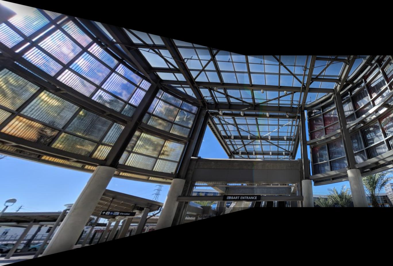
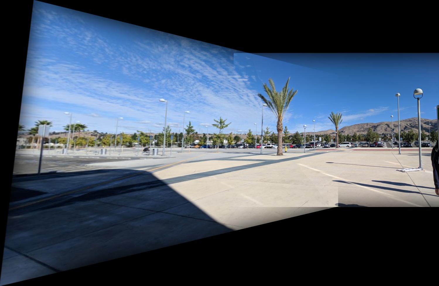
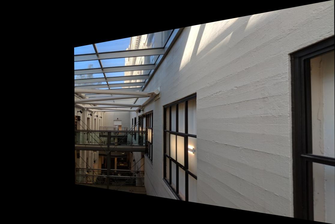
Using the various images I took for mosaics, I then selected a couple of correspondences, warped the images into a common image space, padded the images, and then overlaid and blended the images together.
I ended up creating an ad hoc blending method that uses a Gaussian filter to create a mask that decreases towards the edge of an image. I then used the masks to determine weights in a linear blend of the images. For each pixel, I fix the greater weight and then make sure the other image receives a weight so that the sum of the weights is one.
There are a couple of noticeable artifacts from this blending. For one, you can still see some of the edges towards the top and bottom of the intersection. The second type of artifact is some color splotches caused by the fact that the blending occurred independently on each color channel, and the max function used in blending may have picked different weights in each channel, creating different linear blends for each channel. I had to balance the two types of artifacts: changing the Gaussian filter to make less color splotches would show more of the image edges and vice versa.
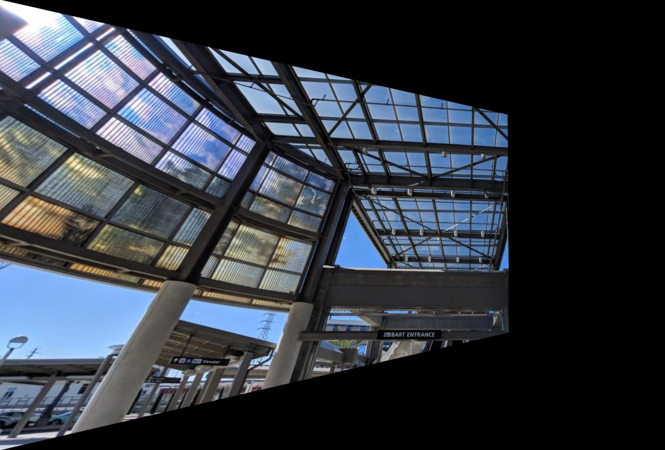
BART Entrance Left Source
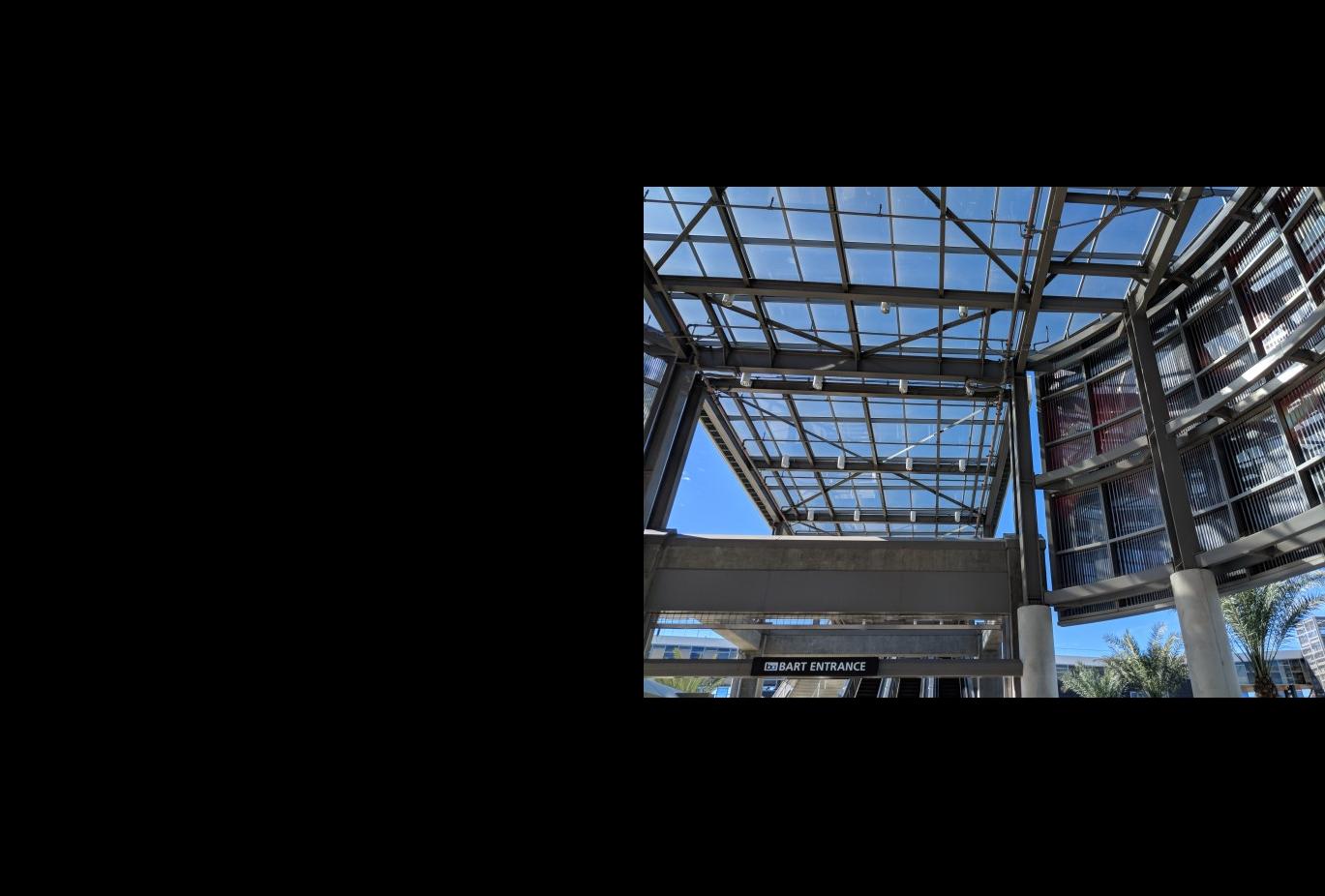
BART Entrance Center Source
BART Entrance Left Padded
BART Entrance Center Padded
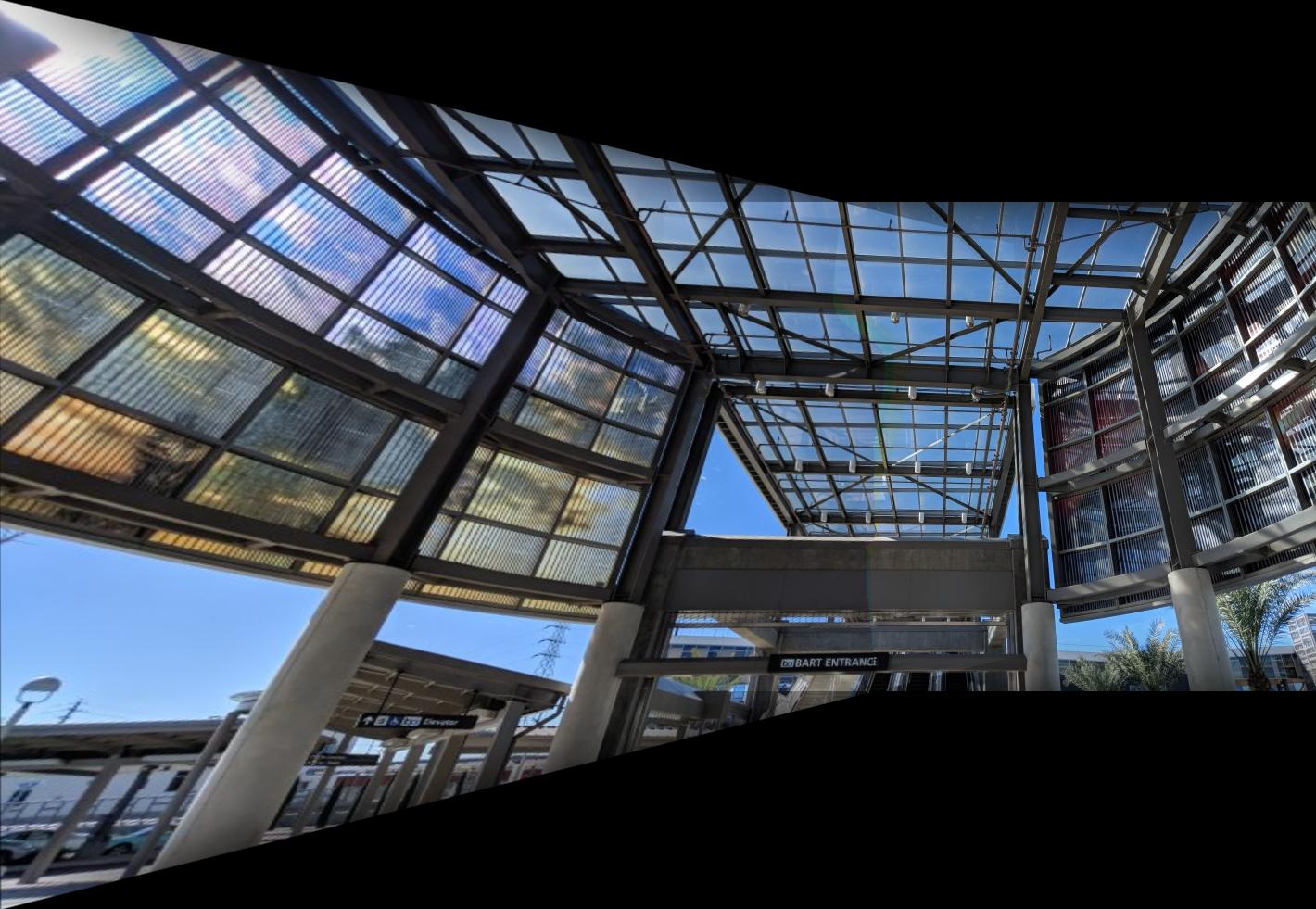
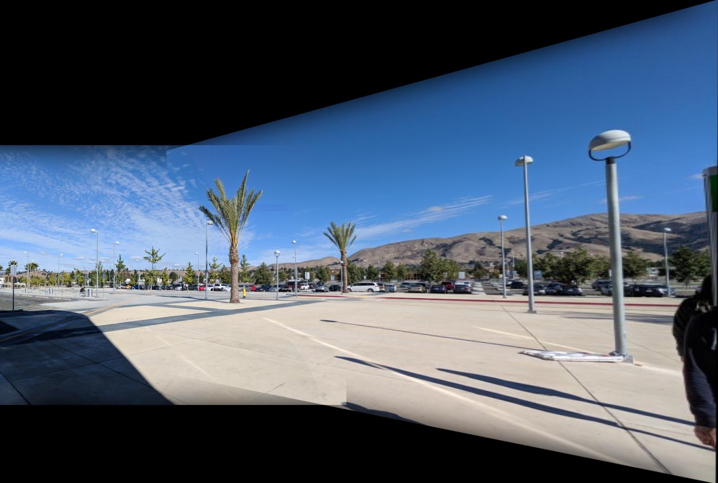
Resulting BART Entrance Mosaic
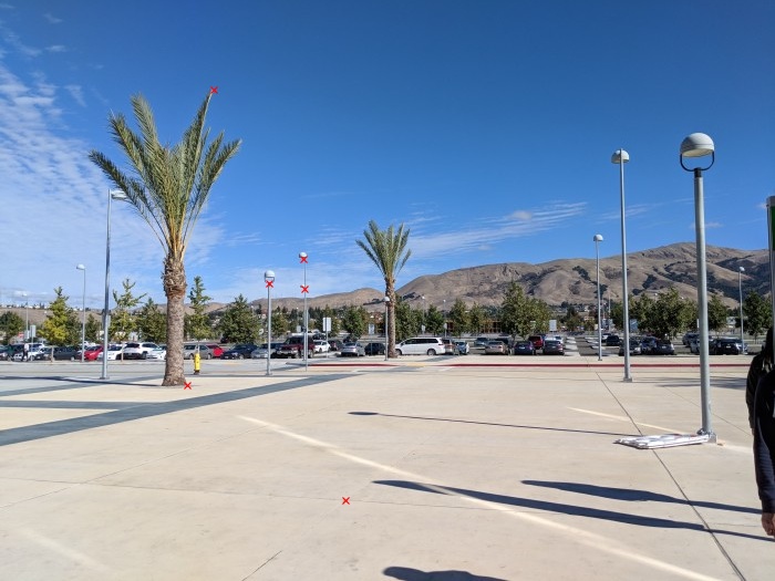
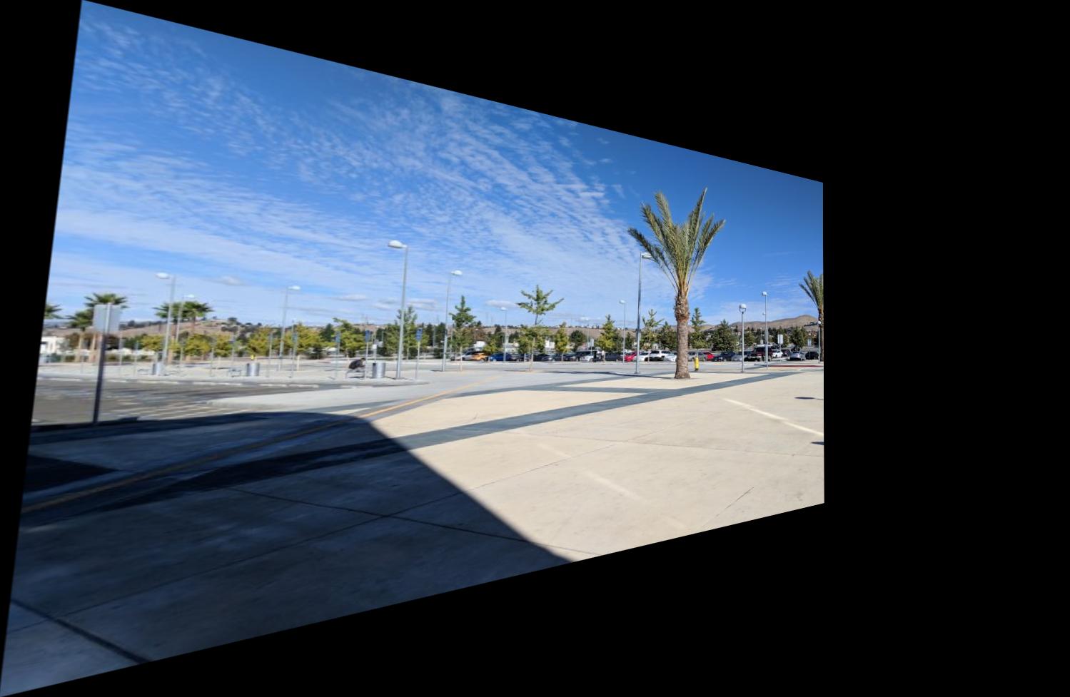
BART Plaza Center Source
BART Plaza Right Source
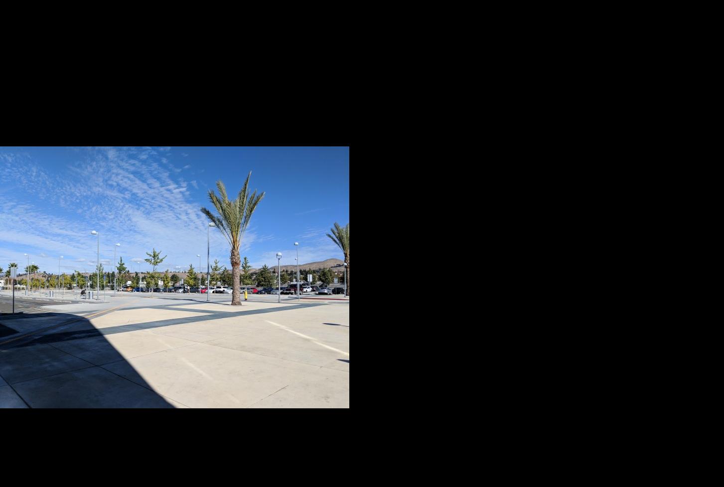
BART Plaza Center Padded
BART Plaza Right Padded
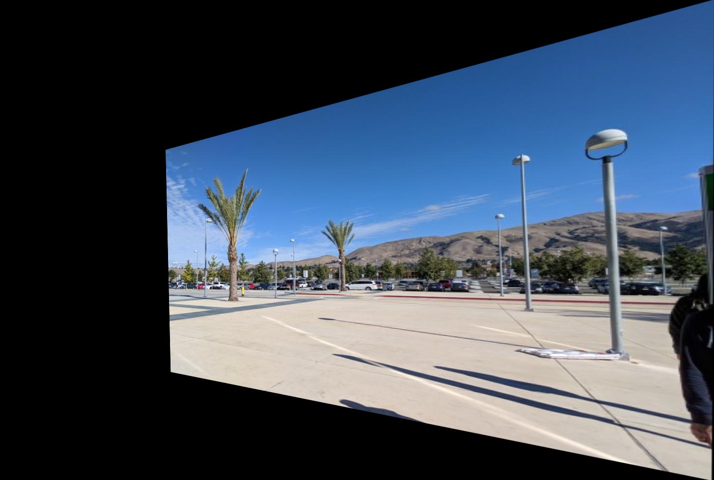
Resulting BART Plaza Mosaic
Library Left Source
Library Center Source
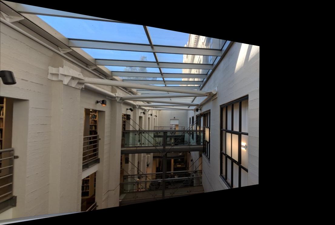
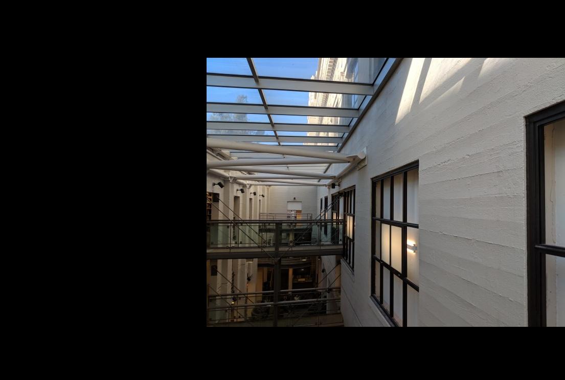
Library Left Padded
Library Center Padded
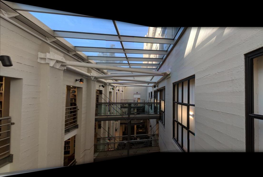
Resulting Library Mosaic
What I Learned
The first thing I learned is that I've reached a dangerous low for my work ethic. I avoided a lot of responsibility which caused me to complete this project pretty late. As a result I was pretty rushed when coding up this project, which may have contributed to more bugs. Additionally, I reached the conclusion that these projects are extremely hard to debug since it's very difficult to narrow down the point of failure.
Regarding the content of the project, I learned that stitching together mosaics is actually remarkably simple and easy. The hardest part is picking a blending algorithm that works and taking pictures that behave well.
CS194-26 Project 6B: Feature Matching for Autostitching
Overview
In this part of the project we simplify methods found in a paper to create code that will automatically detect feature points to stitch images together into a mosaic.
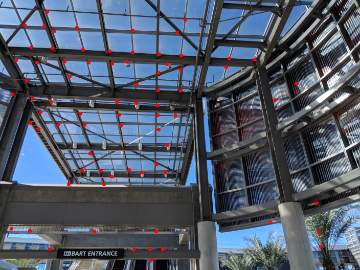
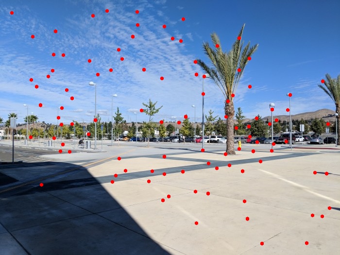
Harris Interest Point Detector
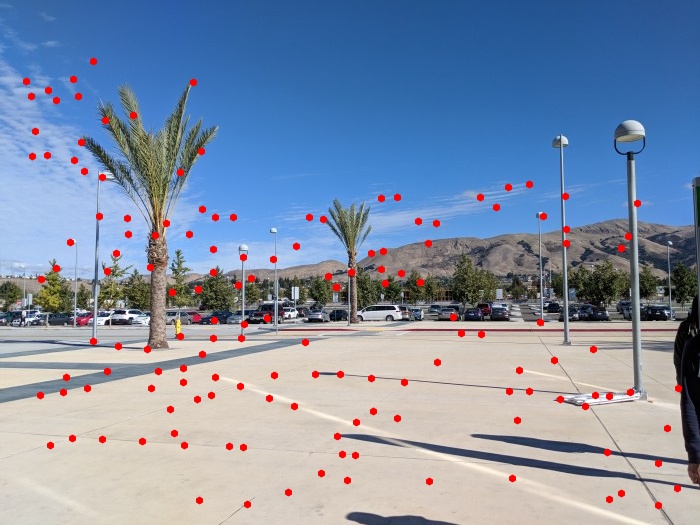
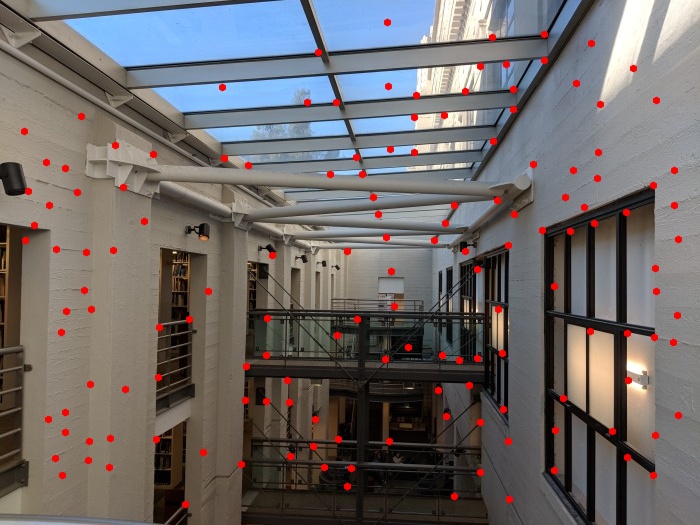
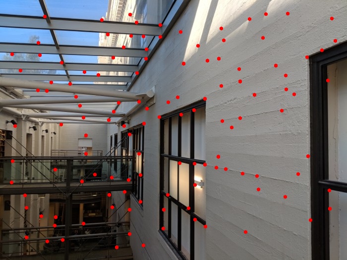
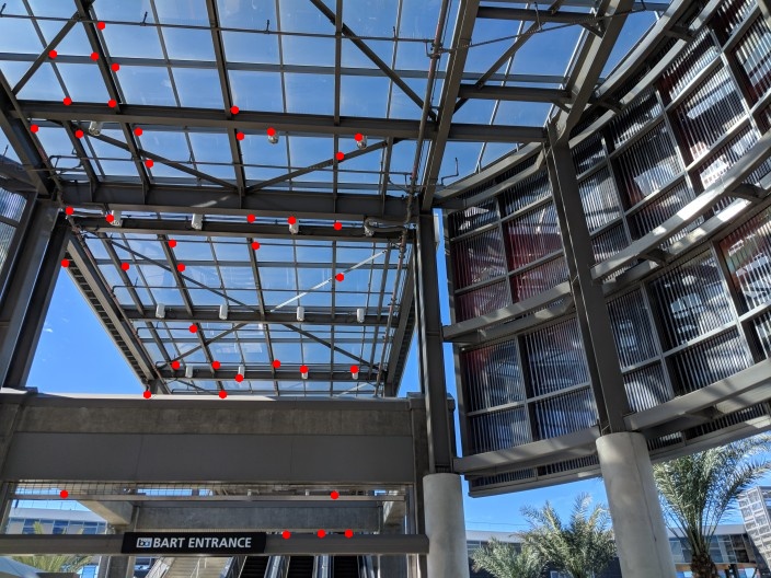
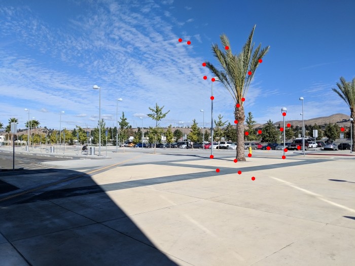
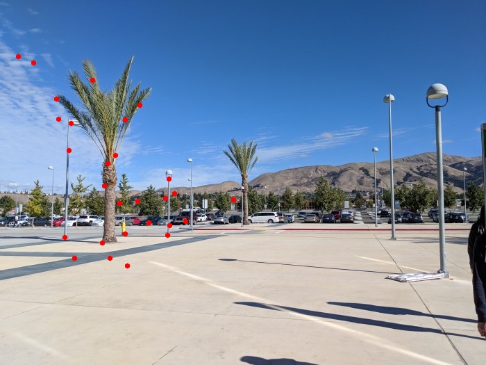
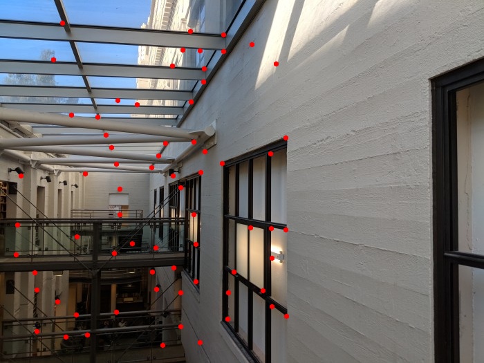
Corners are good feature points in images because they already have a point-like nature and can easily be detected by looking at the gradient of an image. We do detection at a single scale using code that was provided to us. For each position in the image, a Harris matrix (outer product of x and y gradients) is made using pixels surrounding that pixel and then a corner strength is calculated as the harmonic mean of the eigenvalues of the matrix. Below we see our mosaic source images from Part A overlaid with the top 250 corners with the highest corner strength.
Warm Springs/South Fremont BART Entrance Left
Warm Springs/South Fremont BART Entrance Center
Warm Springs/South Fremont BART Plaza Center
Warm Springs/South Fremont BART Plaza Right
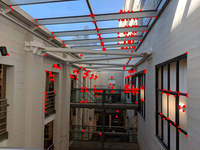
Marian Koshland Bioscience & Natural Resources Library Left
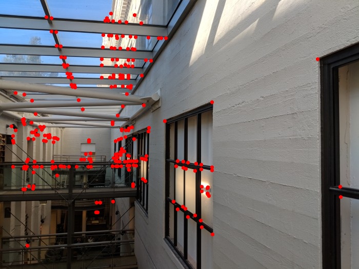
Marian Koshland Bioscience & Natural Resources Library Center
Adaptive Non-Maximal Suppression
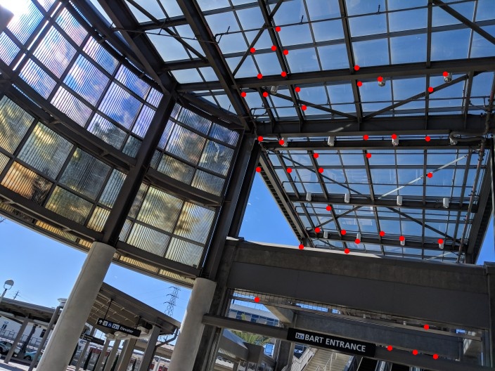
Because we don't know how source images would overlap in a mosaic, we would prefer detected points to be as uniformly spread throughout the image as possible. This would also eliminate some redundancy in detected points that may be trying to identify the same feature. To achieve this, for every detected corner, we calculate the minimum distance to a point whose corner strength is higher by a certain percentage. In our case, we require that the neighbor strength scaled by .9 must be greater than the strength of the original point. We then pick the n features with the greatest distance.
BART Entrance Left, n = 250
BART Entrance Center, n = 250
BART Plaza Center, n = 250
BART Plaza Right, n = 250
Library Left, n = 300
Library Center, n = 300
Feature Descriptors and Matching
For each feature, we create a descriptor. We extract a 8x8 patch of pixels centered around that feature, sampling with a spacing of 5 pixels from a 40x40 pixel window. We then demean the patch and give it a unit standard deviation. To find features that actually correspond in the mosaic, we calculate the squared Euclidean distance between every pair of feature descriptors. Then for every feature and its nearest neighbor, we find the distance between every other descriptor and take the descriptor that produces the lowest 1-NN/2-NN error ratio, and keep the pairing if it's lower than a certain threshold (We use .3).
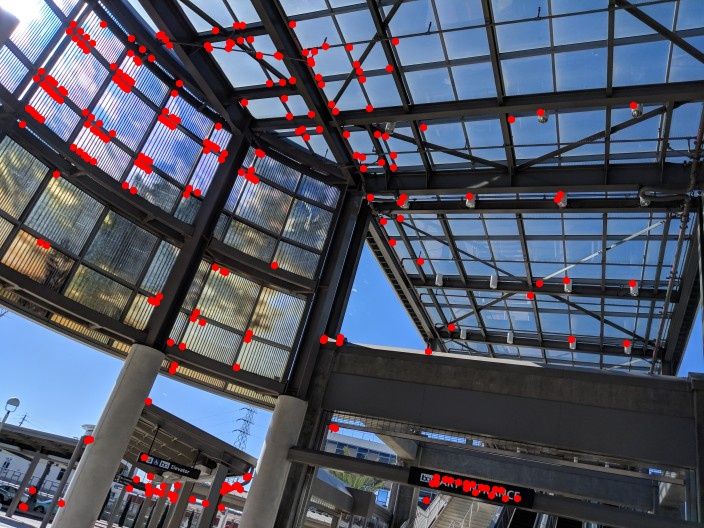
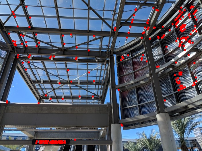
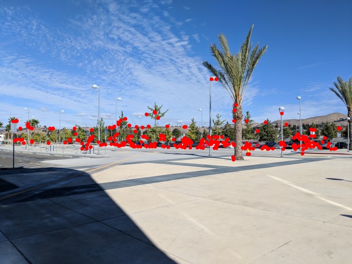
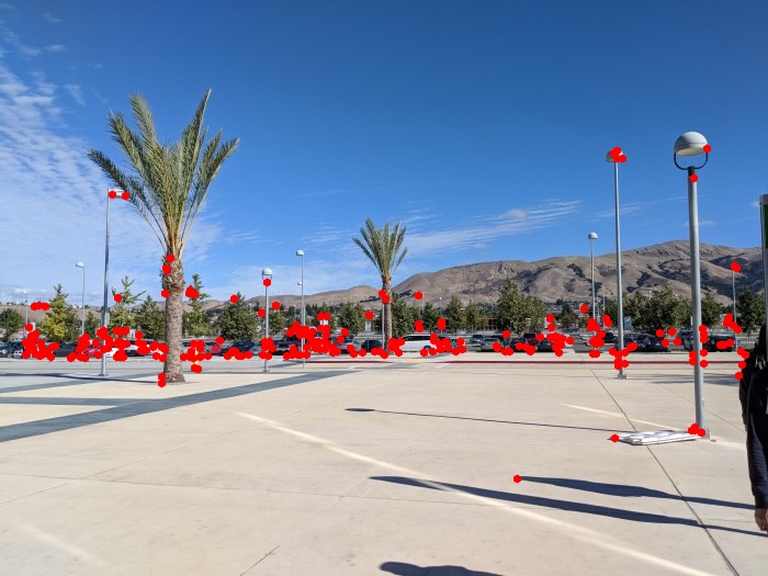
After finding these pairings, we use RANSAC to find the largest set of pairs that agree on a homography, and use those pairs to compute the actual homorgraphy for our pairing. Below, we plot the features kept after running RANSAC for 2000 iterations and an epsilon of 10.
BART Entrance Left
BART Entrance Center
BART Plaza Center
BART Plaza Right
Library Left
Library Center
Mosaics
After doing all the work above, we have automatically found correspondences between our source images and can feed those correspondences to the pipeline form Part A to stitch together our mosaics.
BART Entrance Left Padded
BART Entrance Center Padded
Resulting Automatic BART Entrance Mosaic
Manual BART Entrance Mosaic From Part A
BART Plaza Left Padded
BART Plaza Center Padded
Resulting Automatic BART Plaza Mosaic
Manual BART Plaza Mosaic From Part A
Library Center Padded
Library Right Padded
Resulting Automatic Library Mosaic
Manual Library Mosaic From Part A
What I Learned
Through this project I've learned how simple and easy it is to create something that can automatically stitch together images. However, some of the points picked by the math as features are surprising because they aren't as clear to the human eye (like points in the sky or points that seem to lie on featureless/pointless surfaces or edges). My guess is that they eye and the computer are probably operating on different scales both because of the size of the image and because the code is restricted to looking at smaller local patches of the image.