Overview
How can we take 2 similar pictures of the same scene and cut them together into a continuous photo panorama? Each plane is composed of (x,y) points in a 2D plane, and each picture exists in a different plane. If we can find a transformation from points in one plane to the other, we can align matching features in the 2 pictures and blend the overlapping edges to give the appearance of a single picture. Homographies are 3x3 projective transformation matrices that will allow us to create these transformations.
Part 1: Image Warping and Blending
Image Rectification
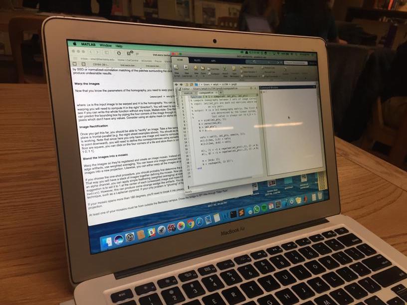
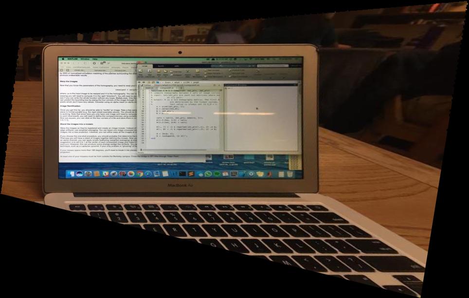
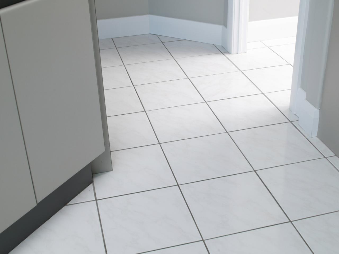
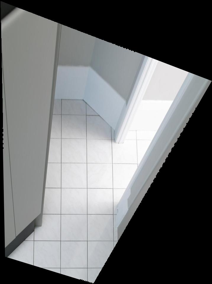
The warmup exercise involves warping a single image from one plane to another. Say a picture contains a view of an object that in real life is square, but because the picture was taken from an angle the object appears trapezoidal. Picking the 4 corners of this object and finding a homography from these points to a unit square (coordinates (0,0), (0,1), (1,1), (1,0)) finds a transformation that "rectifies" an image, making it appear as if the photographer were facing the scene head-on.
Creating the Panorama: Warping
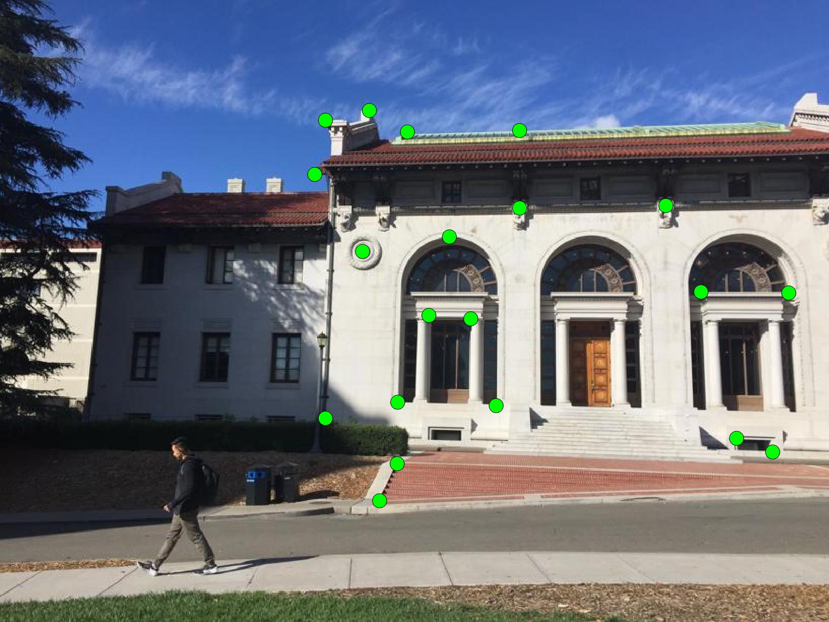
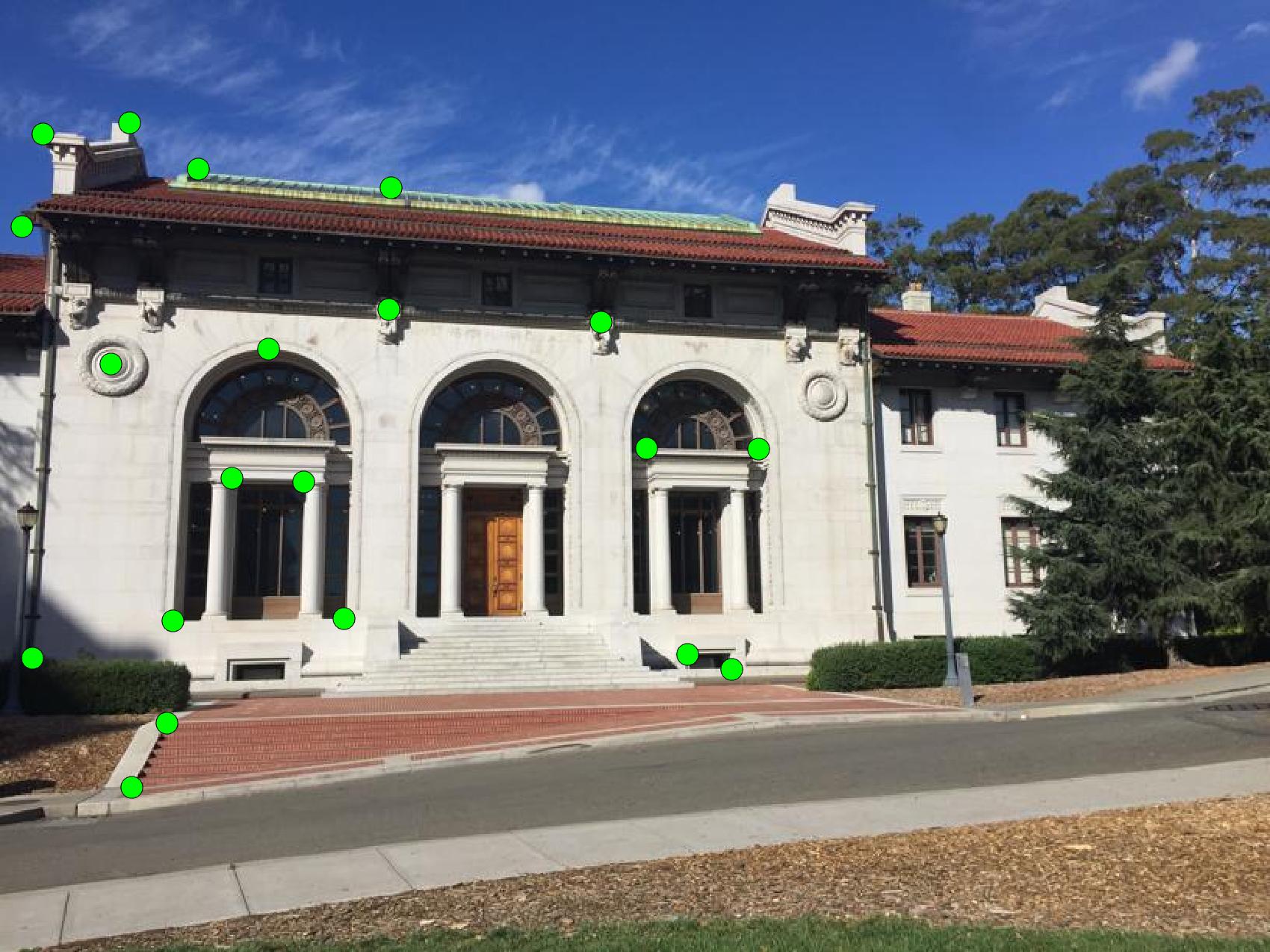
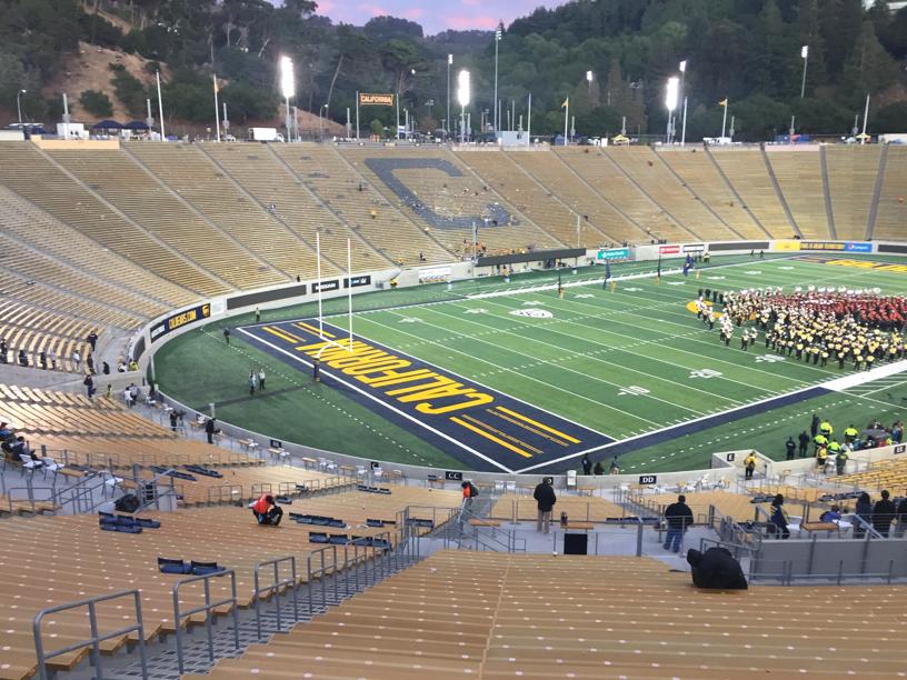
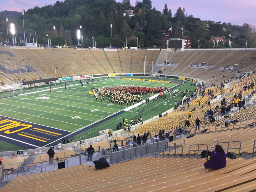
Creating a panorama with 2 separate pictures relies on picking points that refer to the same object/location in both pictures. These reference points "anchor" the transformation, aka if the points chosen to properly capture all the translation and rotation involved from warping from one image to the other, then the estimated homography will also capture all of these transformative properties (or as many as possible, is what we hope for). Instead of forward warping the original image pixels, the coordinates for the new pixels are inverse-warped to coordinates that may lie in between pixels in the original image. If so, the new pixel values are obtained through linear interpolation.
Blending Techniques
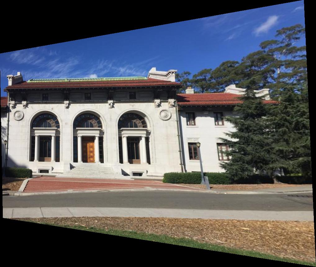
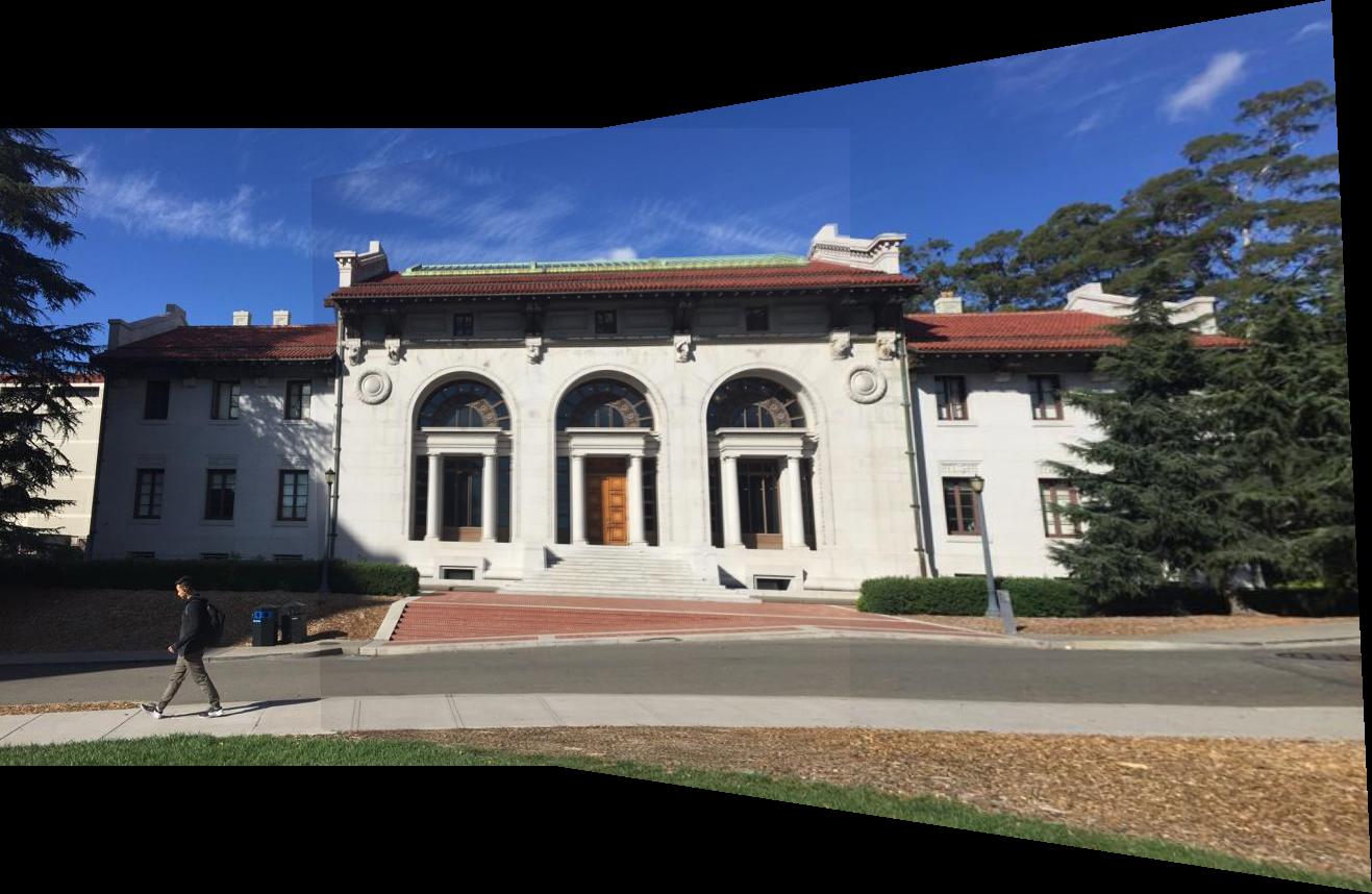
After warping and aligning the 2 images we just need to settle on a technique to blend the the overlaps. The dead simple approch is simply image1 + image2. Pixels outside the overlap region are too dark, and inside the region is too bright, so a quick fix is to create a mask over the entire panorama which is equal to 1/2 in the overlap region, 1 outside the overlap, and 0 elsewhere. This gives even weighting to all pixels in the panorama. The overall look is better, but there are still clear aberrations in the clouds and the right end of the roof.
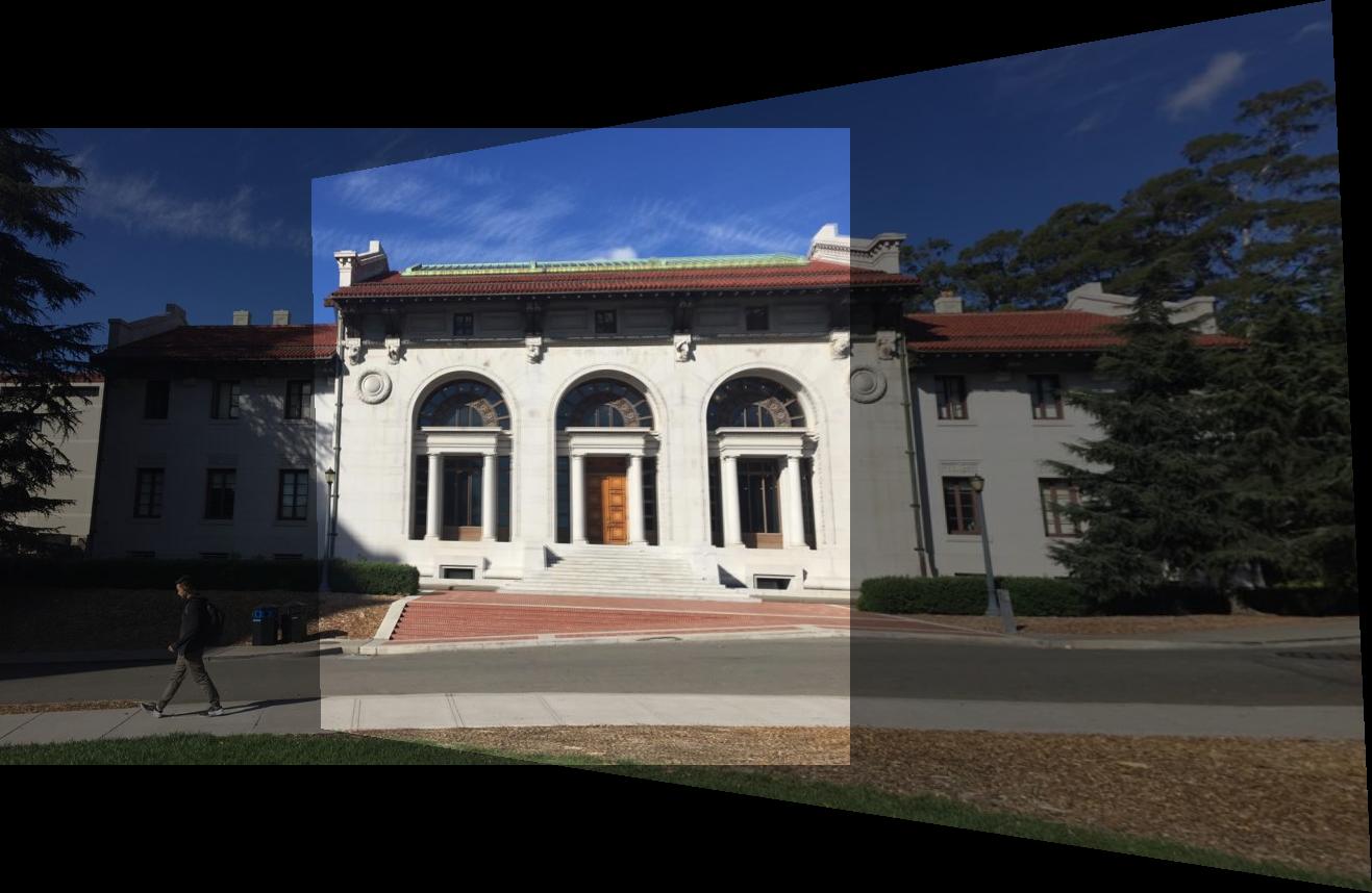
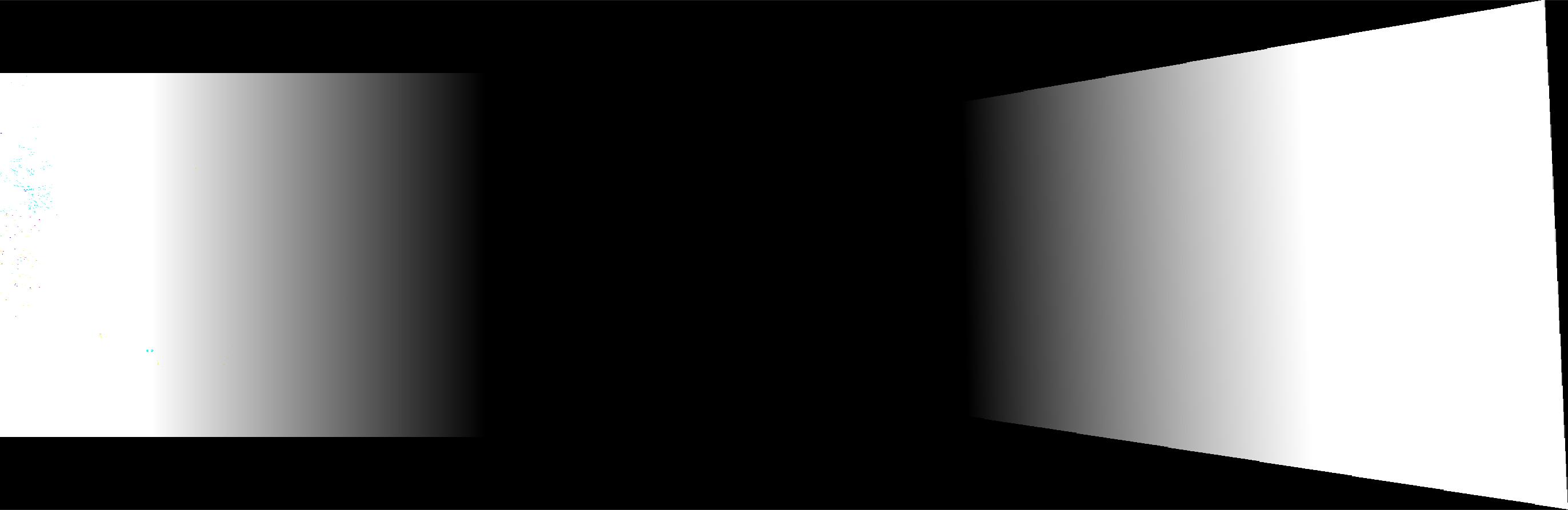
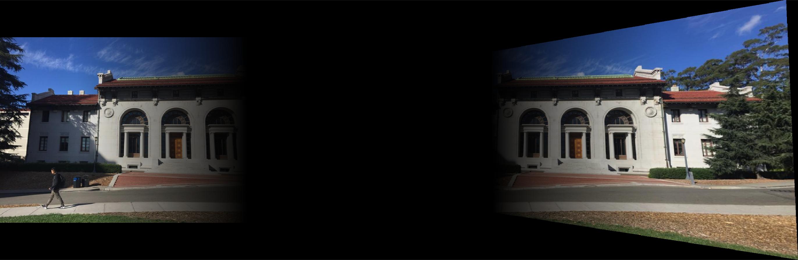
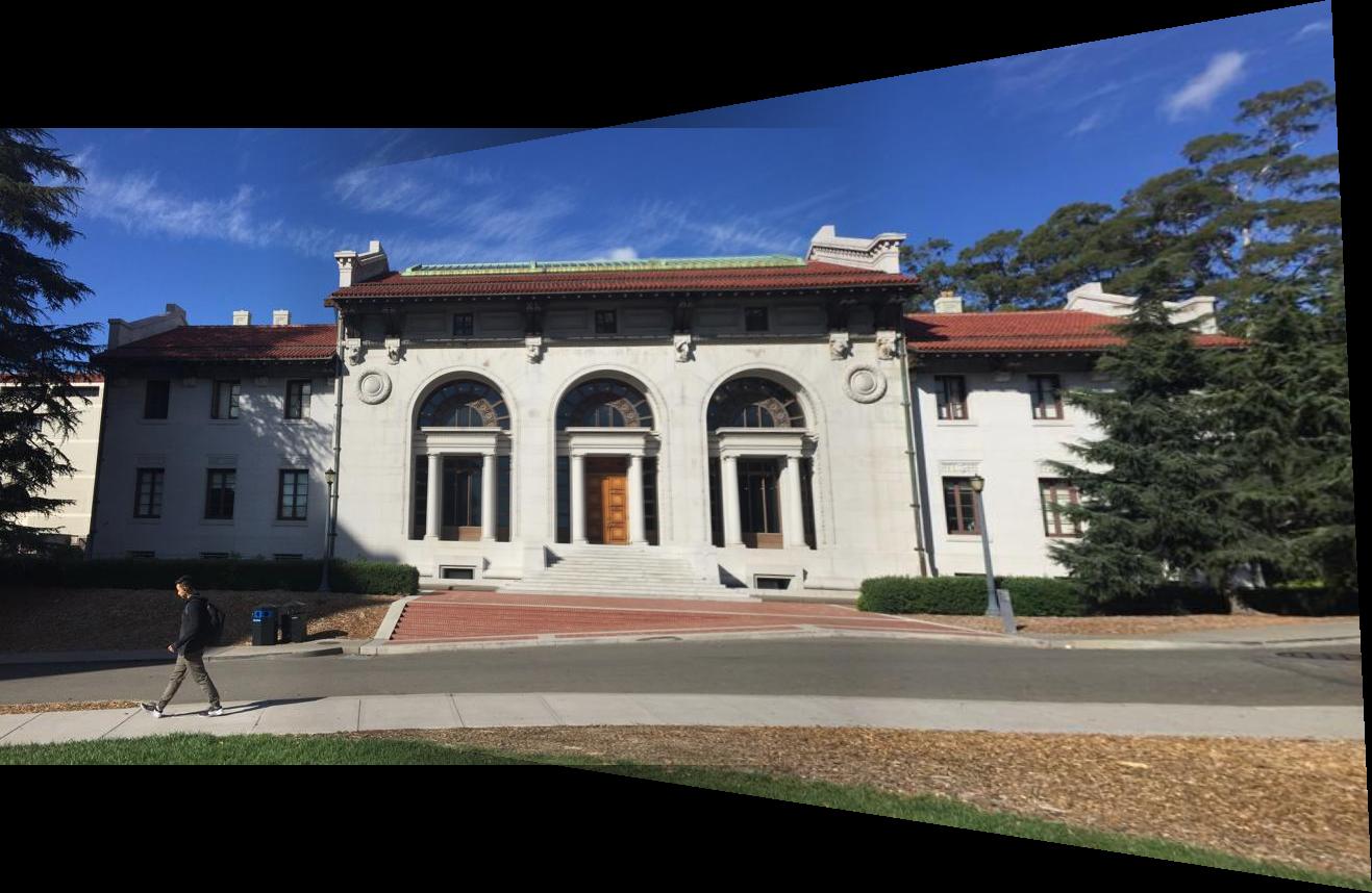
More creative masks yield even better blend results. Linear alpha blending involves creating a mask with an intensity gradient that lets one picture gradually fade out and another fade in at the border where they cross. This completely erases the hard lines seen in the center of the image, but still creates a shadowy effect where the masks intersect. But since these artifacts only occur at the edge, cropping the edges actually produces a very convincing result.
More Results
Part 2: Automatic Point Selection
The results so far have been pretty good, but creating each new panorama is tedious due to the hand-picked point selection process. Enough points must be selected to ensure the homography is robust, but even then a difference of just a few pixels between the corresponding points could lead to catastrophic results. So, this begs the question –
What if we could automate the point selection process?
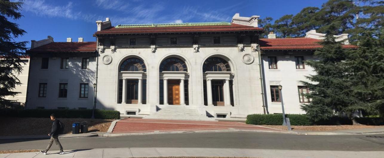
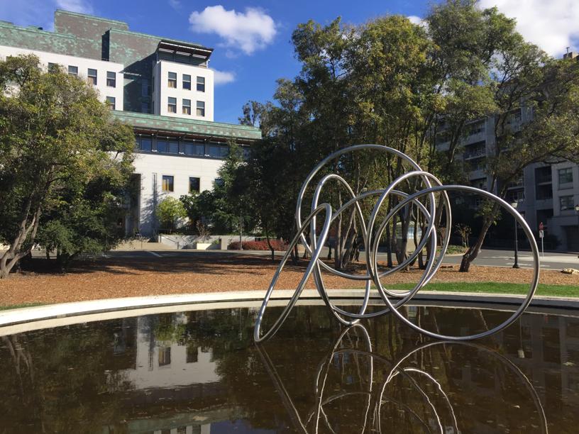
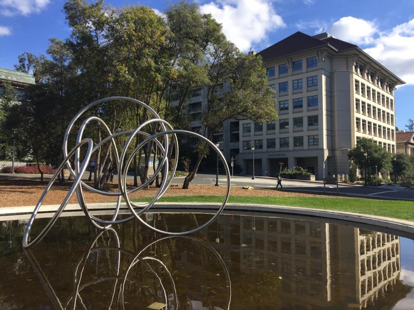
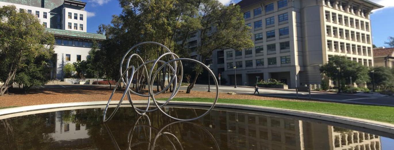
It might sound magical, but with the powers of computer vision and statistical techniques, it's actually feasible and even quite efficient! Many of the methods here were implemented from the paper “Multi-Image Matching using Multi-Scale Oriented Patches”. We'll use these pictures of UC Berkeley's Hearst Mining Circle fountain as an example.
Step 1: Corner Detection
We need exact points to match the images on. Edges are a good metric for aligning entire images, but for exact (x,y) coordinates it's ambiguous which point along the line of the edge is best to use, even in a single imgae. Corners are much more precise and make for a much better metric. In this project corners were located using the Harris Corner Detector (which still ends up using the X/Y gradients of the image to detect corners).
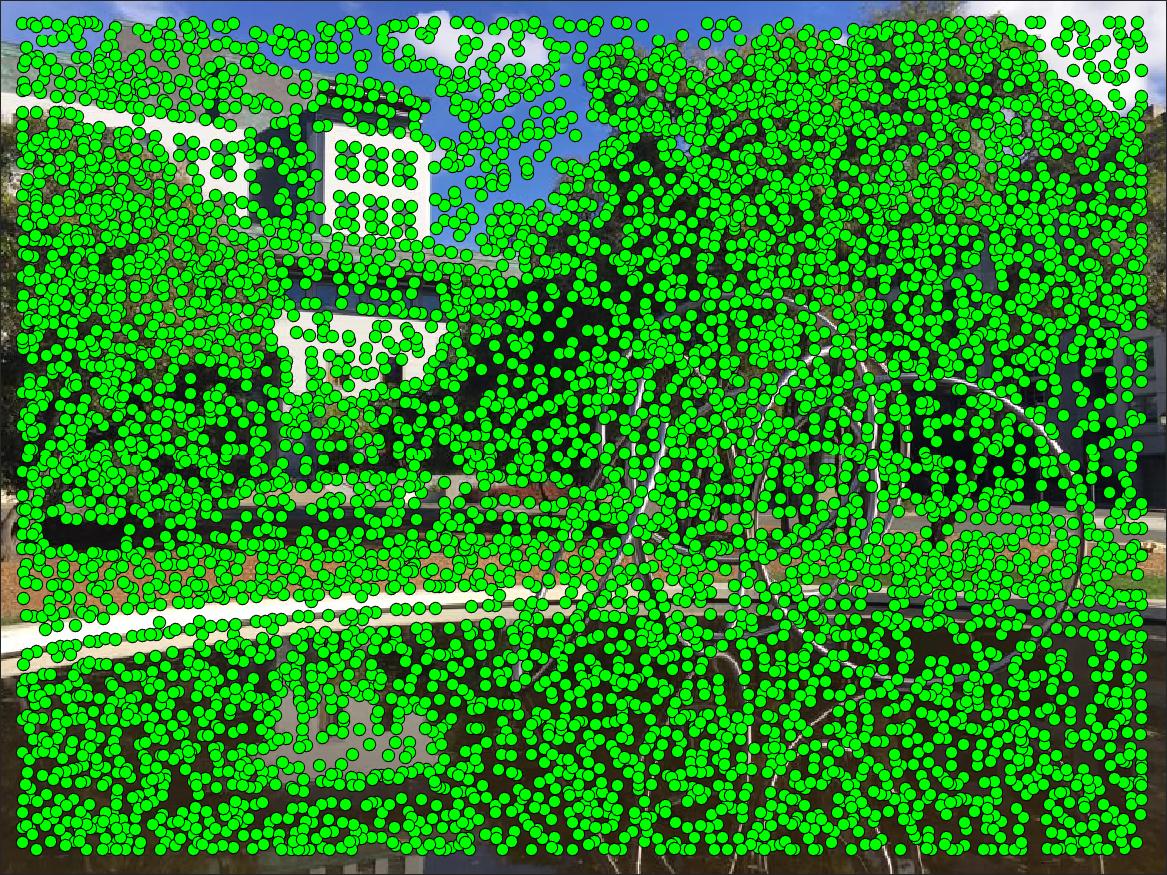
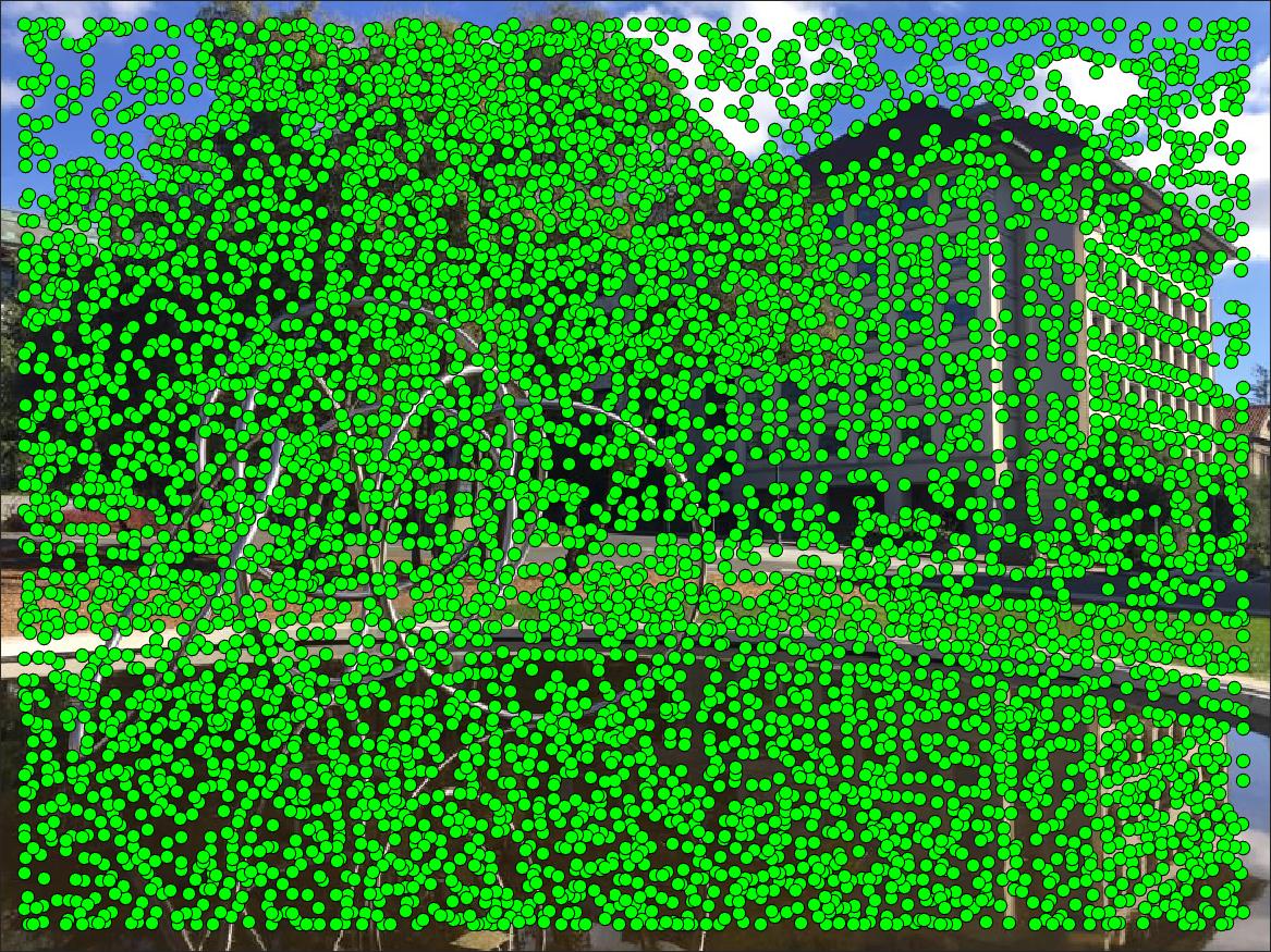
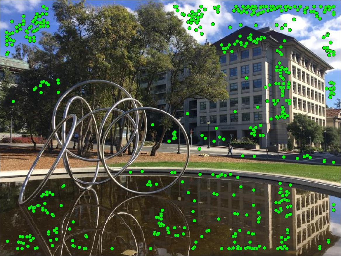
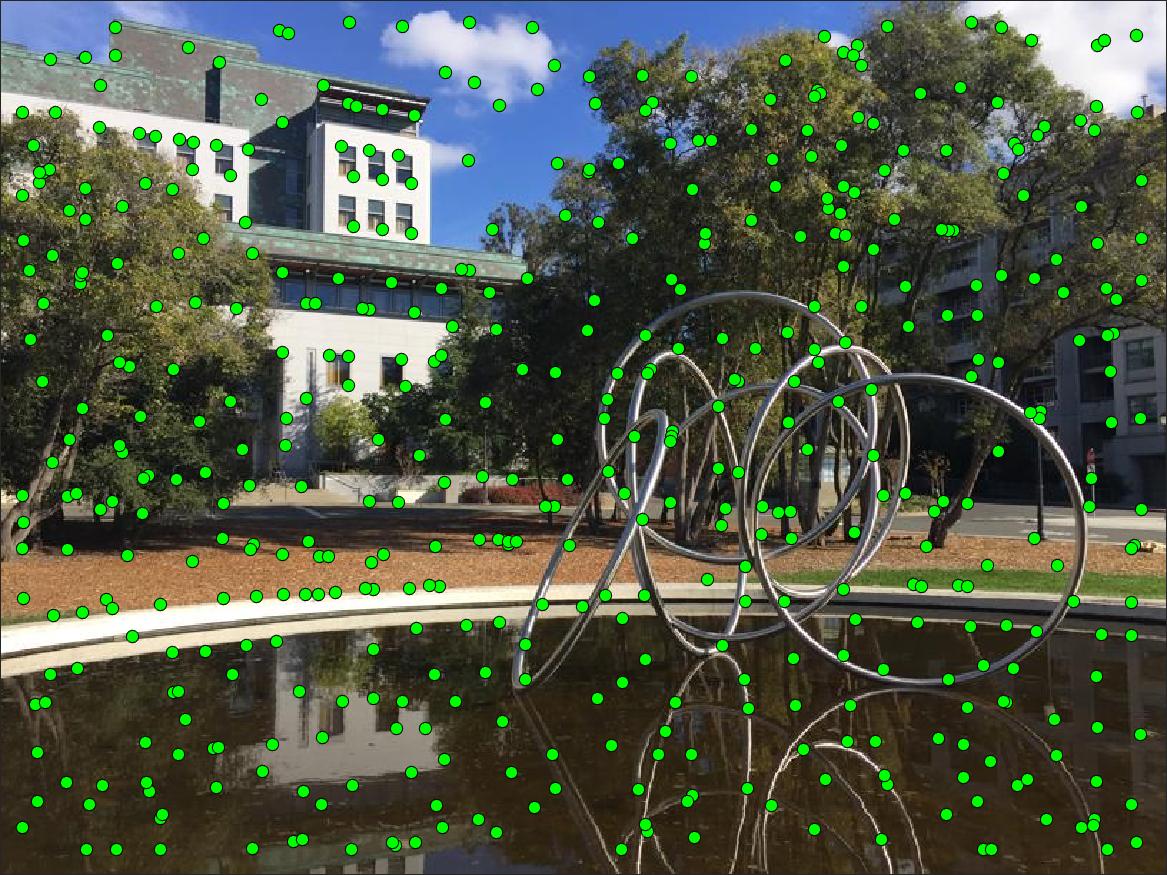
Step 2: Adaptive Non-Maximal Suppression
Corner detection is a good start, but it's clearly overkill - as seen above there are about 6000 corners detected in each image! So the corners need to be filtered somehow. Let's say we want to find N = 500 matching points to create the panorama. Each corner has an associated "corner strength" that is calculated through the detector. One option would be to simply choose the corners with the strongest response from the Harris detector, but this creates a problem as the strongest corners tend to be clustered together.
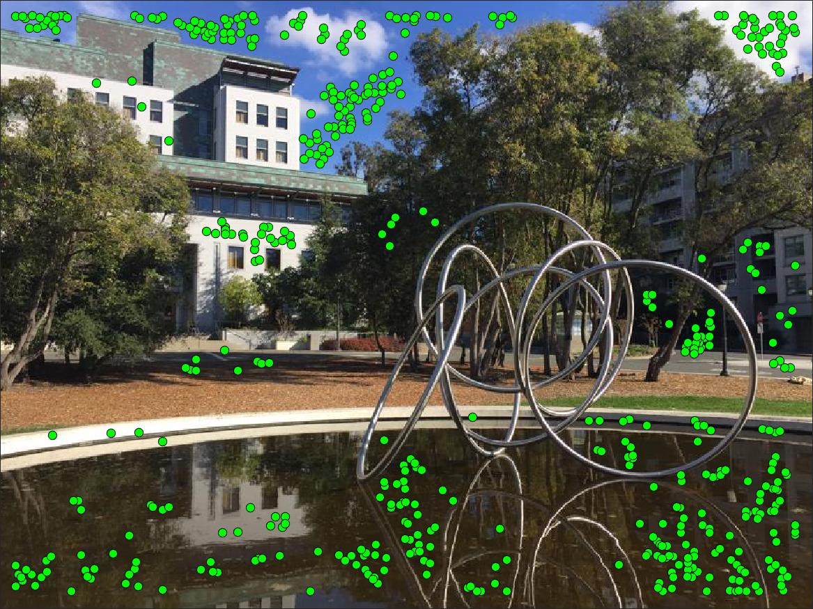
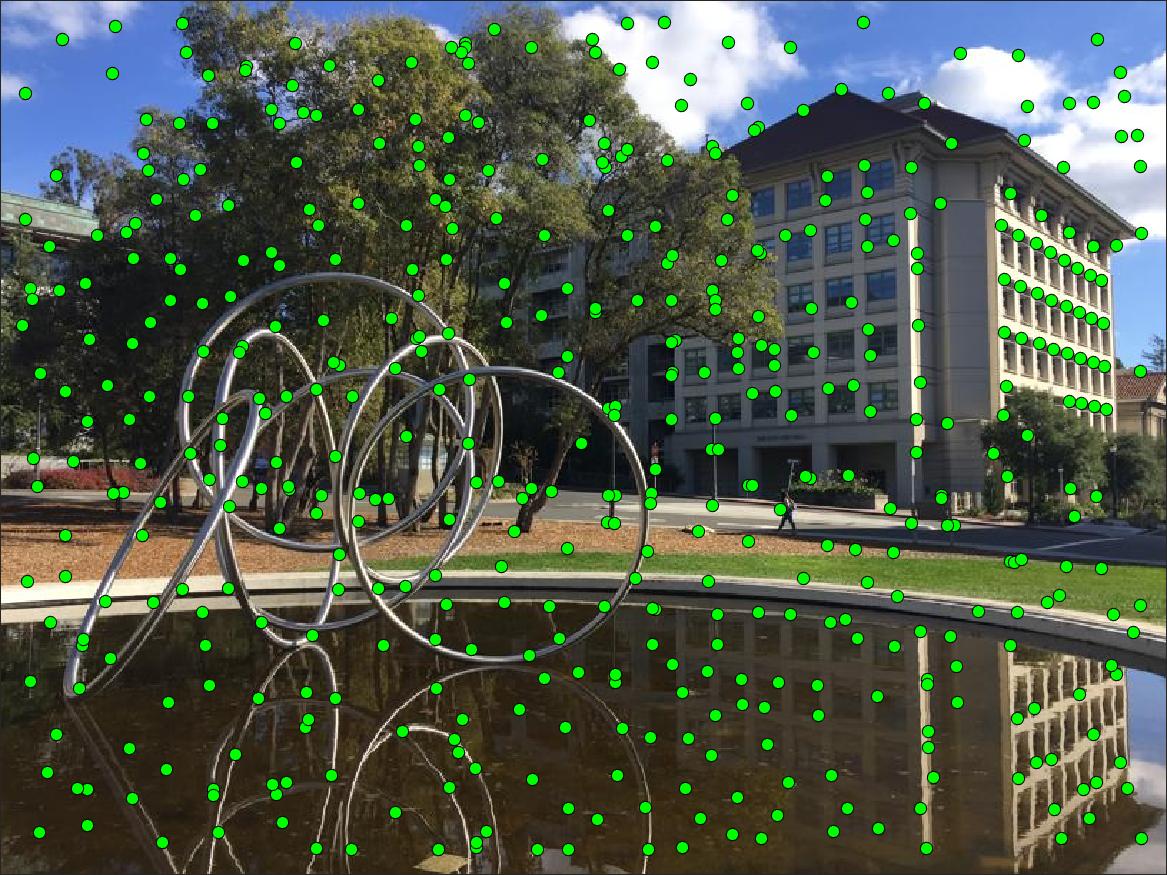
Instead, we apply the method developed by Brown et al. known as Adaptive Non-Maximal Suppression which aims to select more evenly spaced points. The basic idea involves finding, for each point, the smallest radius to a neighboring point that has a corner strength much larger than itself. For example, the point with the globally strongest corner will have a radius of infinity, as no neighboring points are stronger than itself. If we want N points to match on we apply run through ANMS then return points with the N largest "suppression radius" calculated by this method. This means our set of candidates points is an even mix of strong but spaced-out corners.
Step 3: Feature Extraction Matching
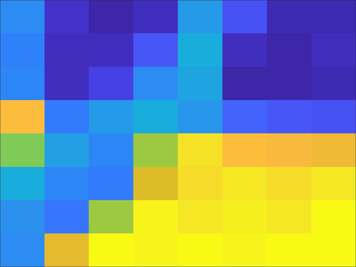
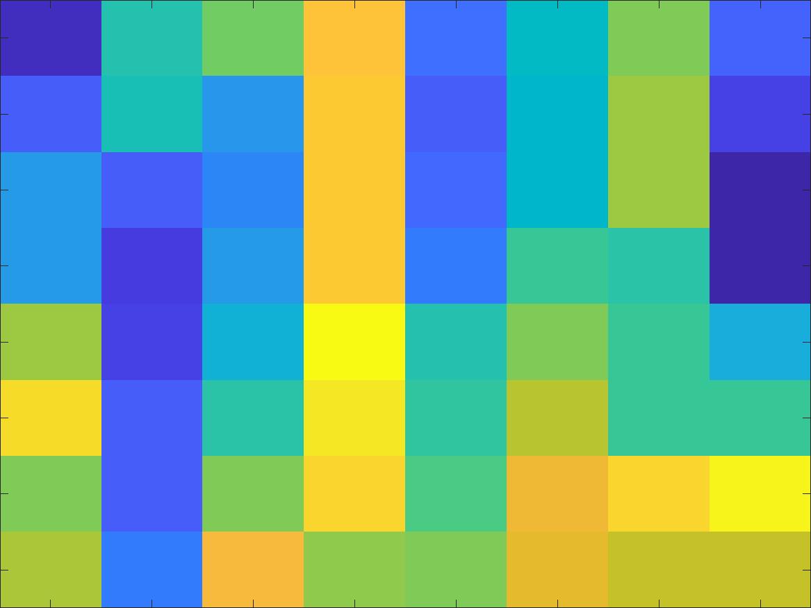
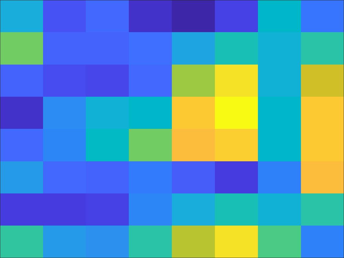
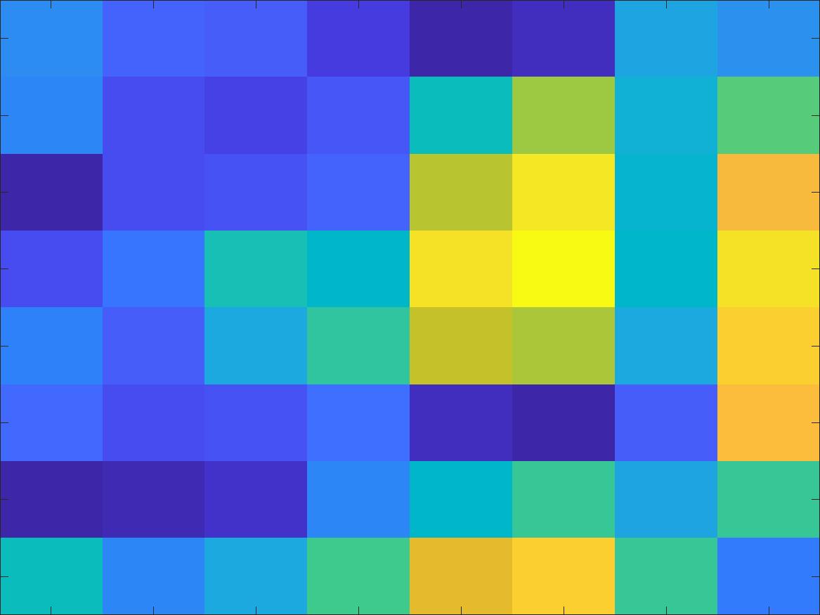
ANMS has given us a good set of candidate points, but we still don't know the correspondene between points in each picture, which the homography estimation is relies on entirely! To do this automatically think about how you as a human would idntify matching points, like the corner of a building. There are multiple buildings with many corners in our example images, but things like the angle of the corner, clouds behind the building, give additional visual context. Programmatically, by taking extractinga a 40x40 pixel window around each point we can do a local comparison, and these windows we use to compare are called features. Additionally, each feature is subsampled and normalized to make the feature invariant to brightness/intensity changes between the images and just focus on the structure.
Some example features are shown below, with the left/right feature taken from the respective image. Looking closely you can notice small differences, so we only keep point pairs whose feature similarity is below a threshold.
Step 4: RANdom SAmple Consensus (RANSAC)
While feature matching is powerful, if even 1 correspondence comes up as a false positive (ie 2 completely different points in the image had similar enough features that they were considered a match) the estimated projection matrix will be completely thrown off. RANSAC helps remove outliers by sampling from the points output by feature matching, computing a homography for these sampled points, then checking how close the homography's projection of image 1 is to image 2. The "inliers" of each estimated homography are again the point pairs that lie under a similarity threshold, and the largest set of inliers is used to create the final homography matrix.
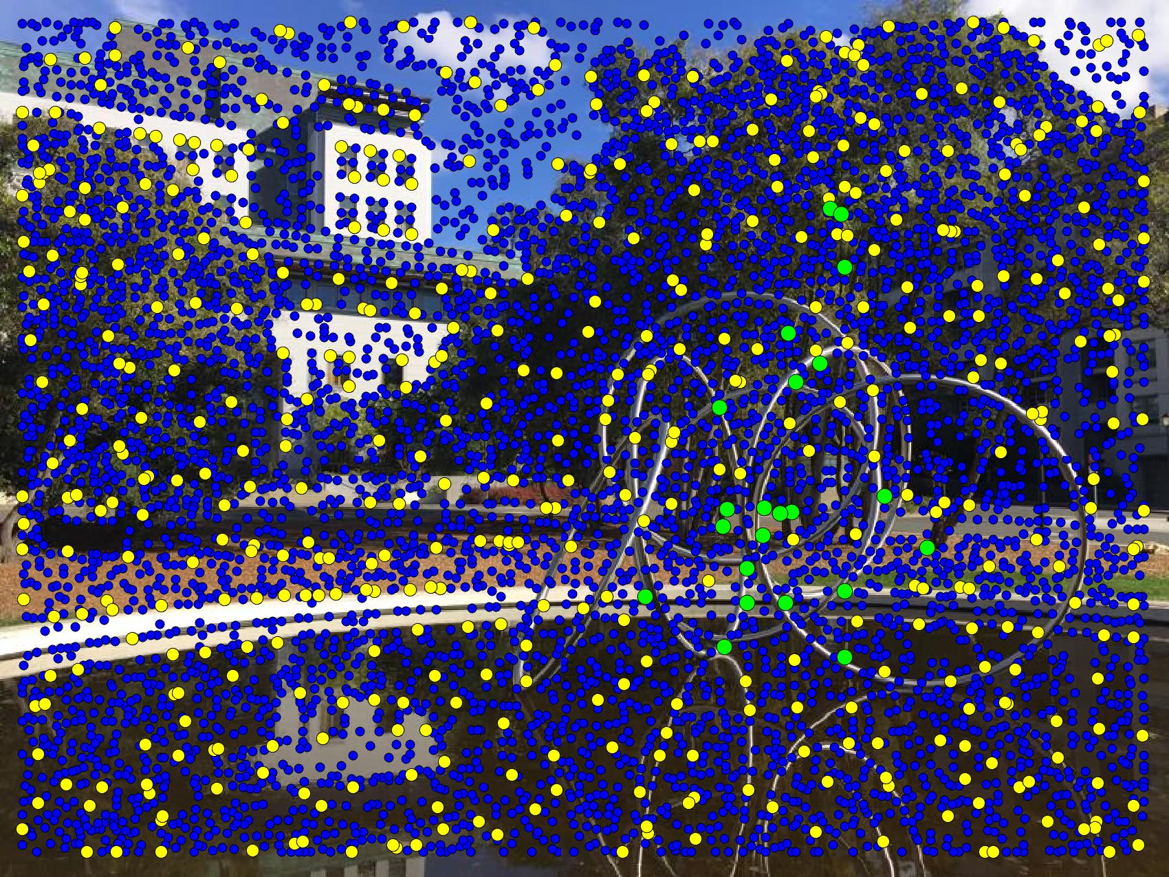
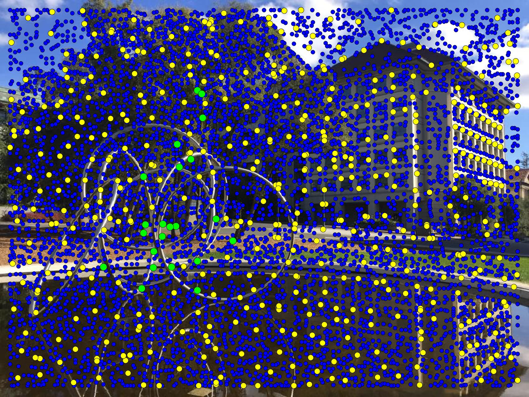
The images below show the process of filtering out candidate points through the steps mentioned above. This entire process, even with 10,000 iterations of RANSAC, took barely 3 seconds to go through this entire process for 612x816 images, and about 30 seconds for images double that resolution.
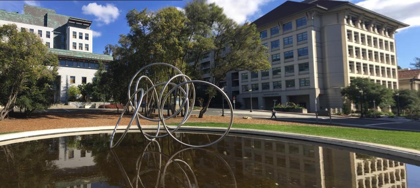
Results!
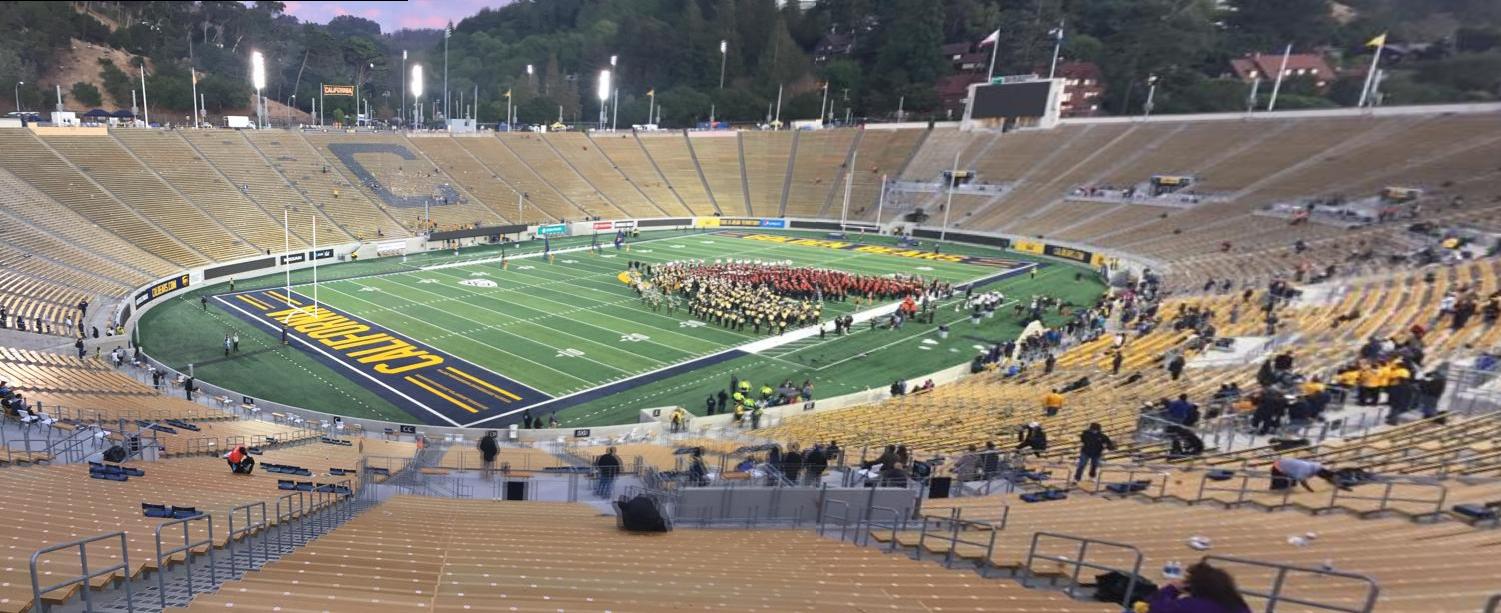
After applying the same warping/blending techniques from Part 1, we now have a full pipeline that will pick out matching points, compute and apply a projective homography, and blend and crop the results to create amazing panoramos. I'm still amazed at the results as I'm typing this out!!
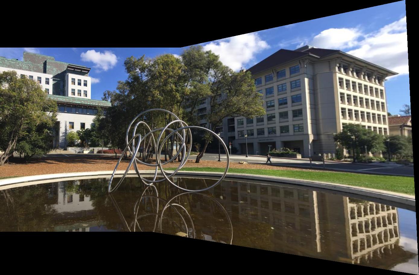
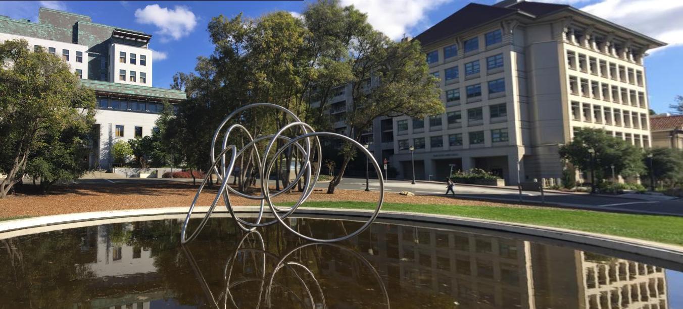
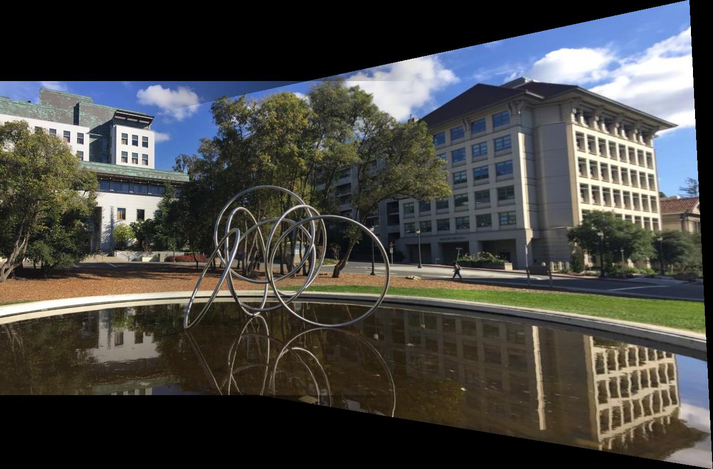

Comparing the 2 Methods
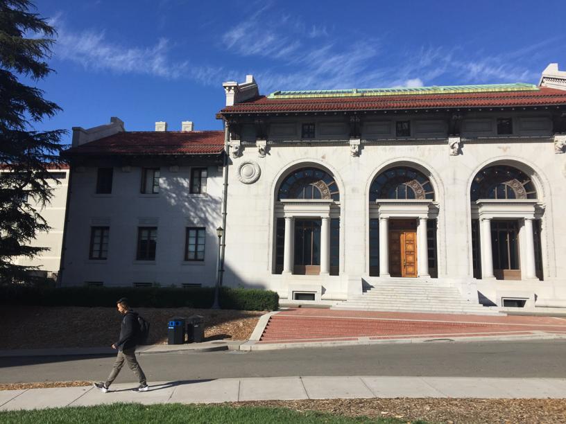
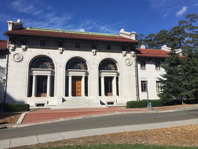
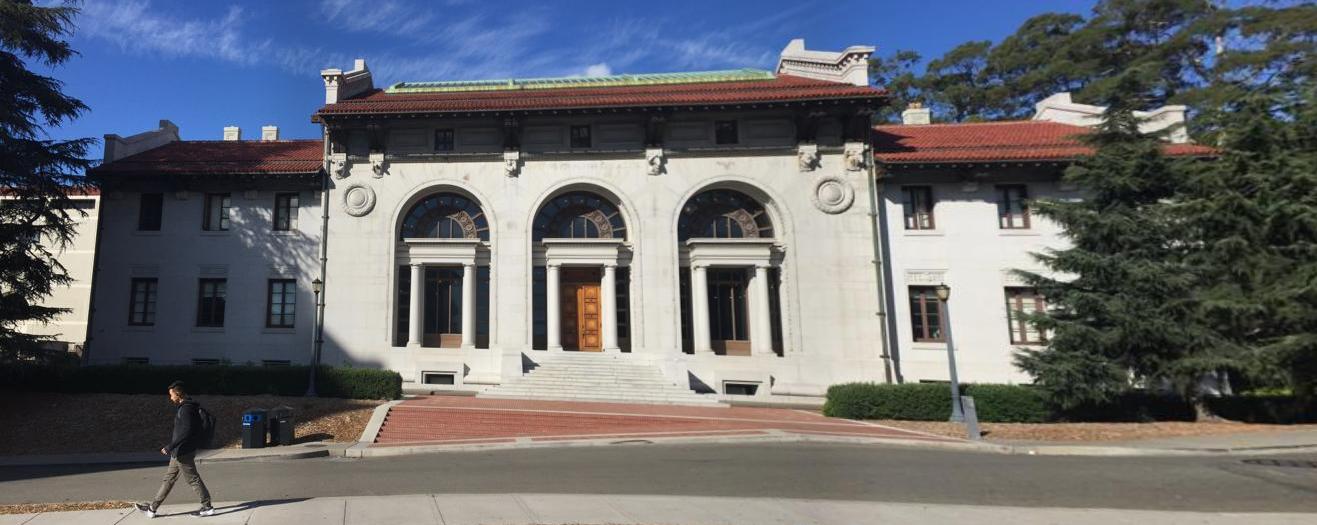
(The front door to the building is less blurry)
What I Learned
Every part of the automation process was amazing to me. The idea of sampling/blurring the features to make them invariant to image noise, the robustness of RANSAC, each step is not terribly hard to comprehend but all put together they are incredibly powerful!! As for the homography transformations, I am continually impressed with the power of least squares. I'm actually excited to try testing the limits of this system on more and more photographs that I take in the future.