Project #6: [Auto]Stitching Photo Mosaics

Part A

Overview

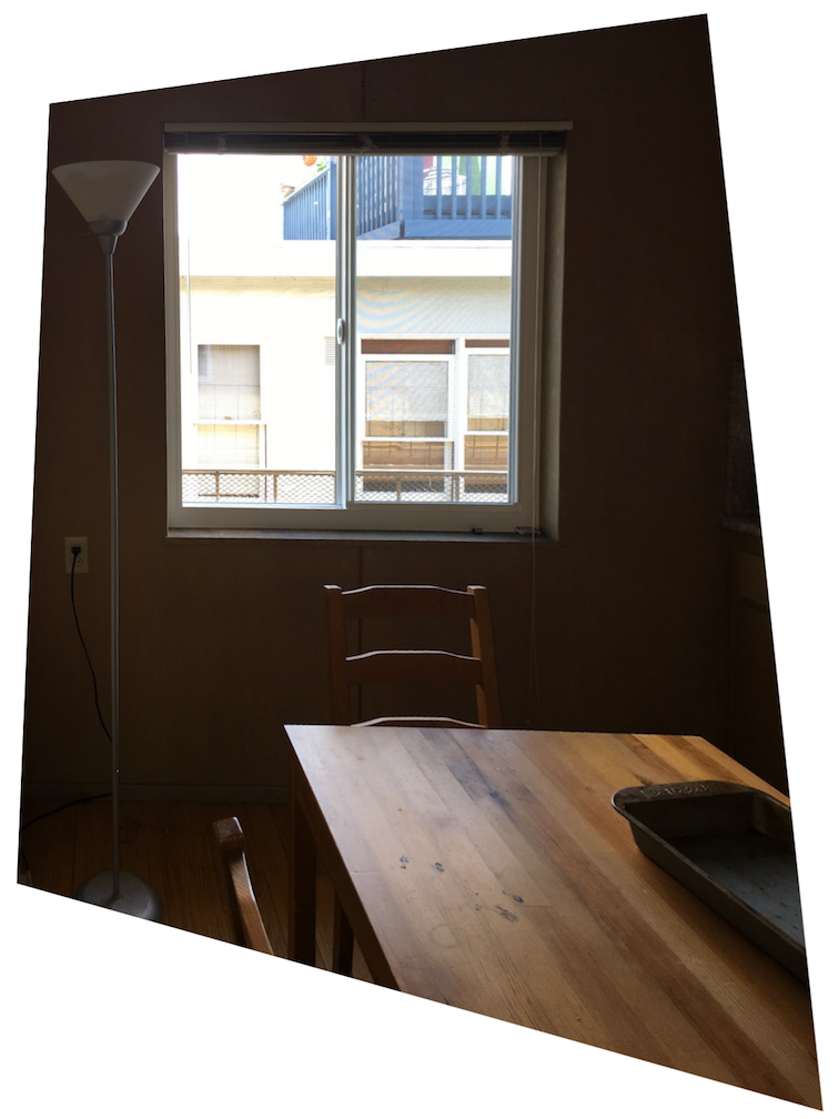
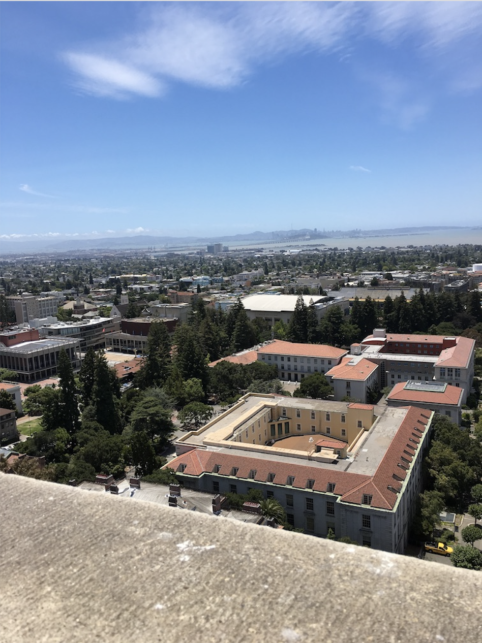
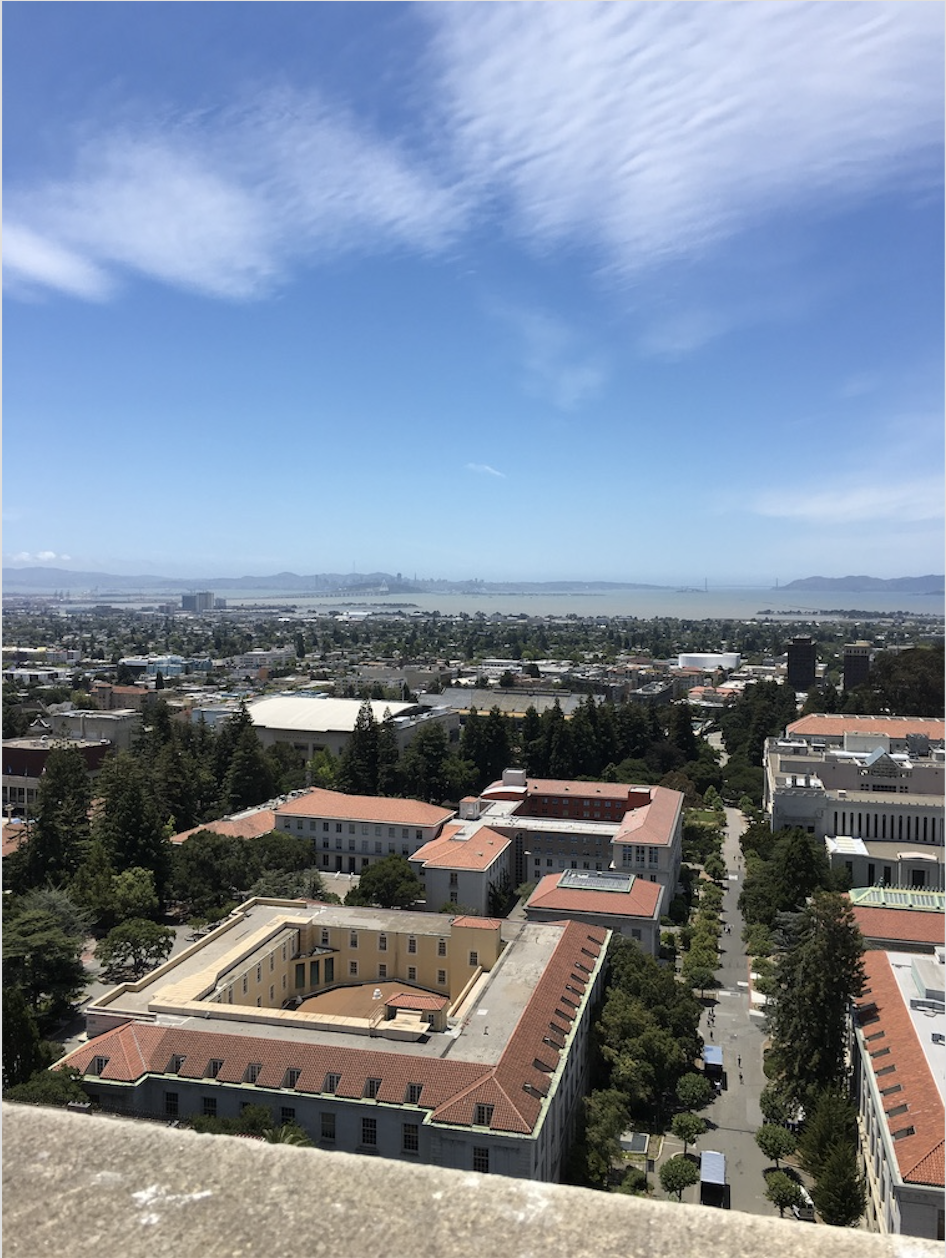
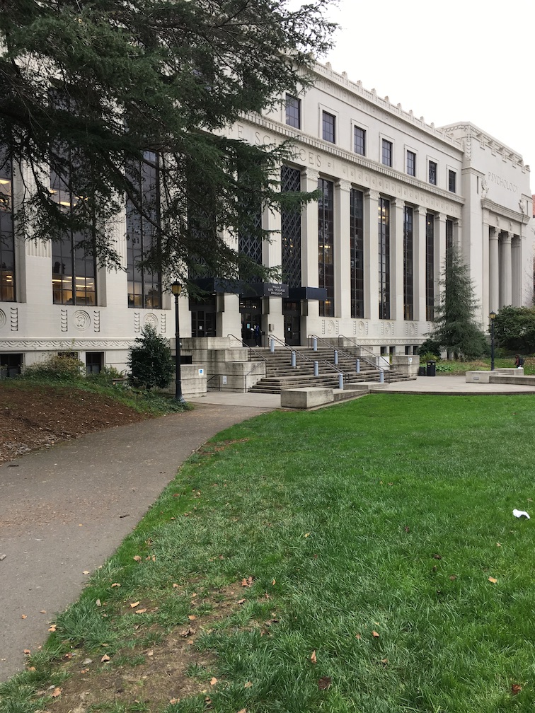
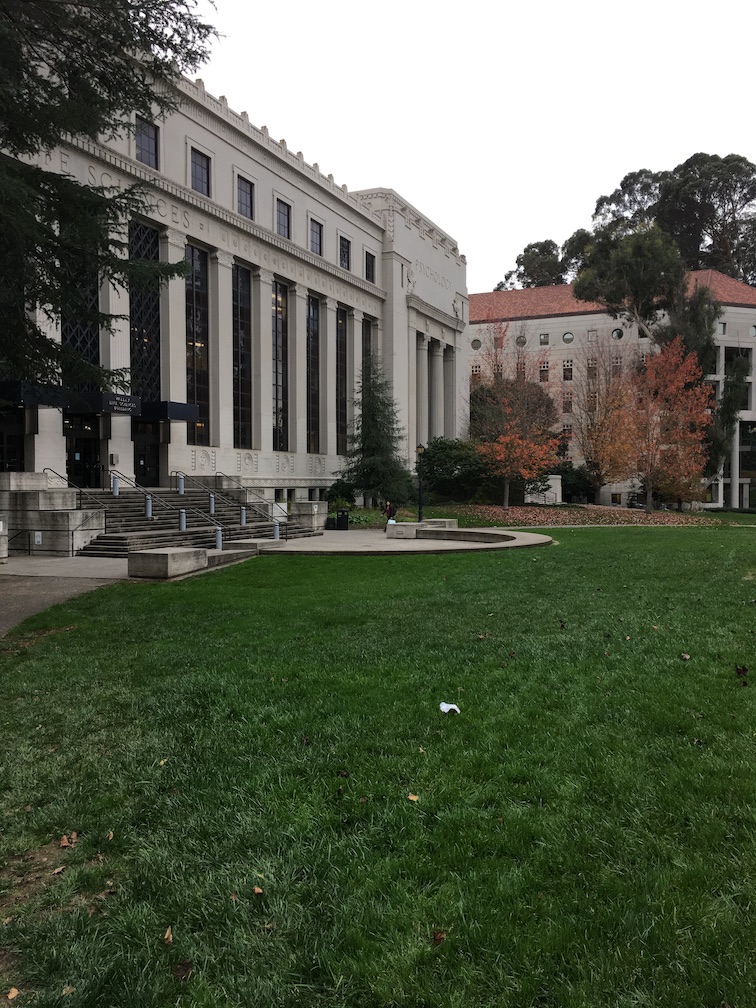
The goal of this project is to compute homographies between images and warp them into rectified images and mosaics. In order to do this, I captured images from the same point of view but with different view directions. Then, the homography transformation matrix is recovered by selecting corresponding points between pairs of images.

Recover Homographies

Corresponding points can be related via a single 3x3 matrix. Another way to express this point is by p' = Hp where H is a 3x3 matrix with 9 parameters. Since the last parameter is a scaling factor, we can fix it to 1 and solve for the other 8 parameters via a linear system of equations. If we rearrange the problem to solve for the 8 parameters, we know that we only need 4 points (of 2 coordinates each) to completely determine the system. However, since we are picking these points by hand, there is bound to be error, thus I collected 10-15 points for each pair of images and solved the system by linear least squares. Once H is recovered, I use inverse warping to transform the second image to the desired perspective.

Image Rectification

I start by rectifying images using this technique so that they are frontal parallel. I have two examples for this part. In the first, I try to rectify the image so that the window is frontal parallel. As you can see, the rectified image isn't perfect since the table does not appear frontal parallel. Throwing more points into our system of equations could improve the results. However, it is difficult to specify where the target points without a real frontal parallel image as reference. In the second example, I warp the image so that the construction sign is frontal parallel.

Original

Rectified

Original

Rectified

Blending the Images into a Mosaic

In this section, I warp several images into mosaics by computing the homographies. I use linear blending to create a seamless composition. In the first example, you can see that the warping is imperfect. In fact, on the right half of the mosaic, you can clearly see an artifact. I had taken the picture while a person wearing red was walking along this pictured path!

Source 1

Source 2

Source 3

Outside of VLSB

Source 1

Source 2

Source 3

On Top of the Campanile

Source 1

Source 2

North Beach of San Francisco

Summary

In this project, I learned how easily images can be stitched together using homographies. This is an incredibly cool and simple concept that is widely used today.

Part B

Overview

The goal of this project is to automatically detect matching features to compute the homographies described in the previous part. In order to do so, we will find Harris corners and find matching features by computing the SSD of their feature descriptors.

Harris Interest Point Detector

The first step is to find Harris corners to find interest points.

Harris Corners in Source 1

Harris Corners in Source 2

Harris Corners in Source 3

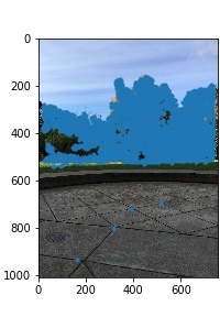
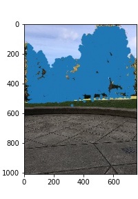
Adaptive Non-Maximal Suppression

In the next step, we suppress the number of feature points by calculating the distance to the nearest neighboring point with a higher Harris intensity. Then, I sorted the points by these distances and picked the top 200.

Suppressed Points in Source 1

Suppressed Points in Source 2

Suppressed Points in Source 3

Feature Descriptor Extraction and Feature Matching

Next, we extract axis-aligned 8x8 patches for each of the feature points found in the previous step. These patches are sampled from a larger 40x40 window with spacing of 5 pixels. For each pair of patch from the first image, we find the best two patches from the second image and calculate the ratio of the SSD of the best match and the SSD of the second best match. If this ratio was less than 0.3, we conclude that this is a good match.

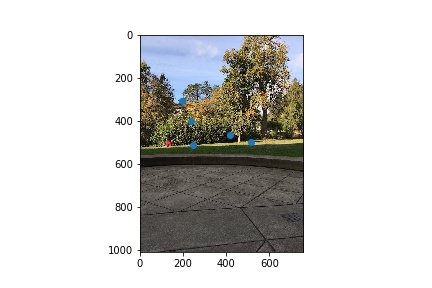
Matching Features in Source 2

Matching Features in Source 3

RANSAC

In the final step, we use RANSAC to further filter out bad feature points. For 1000 iterations, we sample 4 points from the matching features found in the previous step and estimate a homography. We then use this homography to estimate the transformation of the feature points in the first image and count the number of inliers where an inlier is defined to be a feature point that has a Euclidean distance smaller than 5 to the estimated point from the computed homography. At the end, we pick the largest set of inliers and compute a new homography with this set of inlier points. This homography is used to warp the first image.

Source 1

Source 2

Source 3

Manually Stitched Mosaic (Cropped)

Automatically Stitched Mosaic

In the manual stitching, the corresponding points were mostly on the ground. Thus, the first mosaic is extremely aligned in the bottom half of the stitch. In the automatic alignment, the detected features were in the top half of the images and thus we see some ghosting in the bottom half of the stitch specifically in the tiles. However, the automatic stitch is much better as there is no seam in the right half of the image anymore.

Source 1

Source 2

Manually Stitched Mosaic with 3 Sources (Cropped)

Automatically Stitched Mosaic

The third image did not stitch well here because of a lack of matching feature points detected.

Source 1

Source 2

Source 3

Outside of VLSB 2

Source 1

Source 2

Source 3

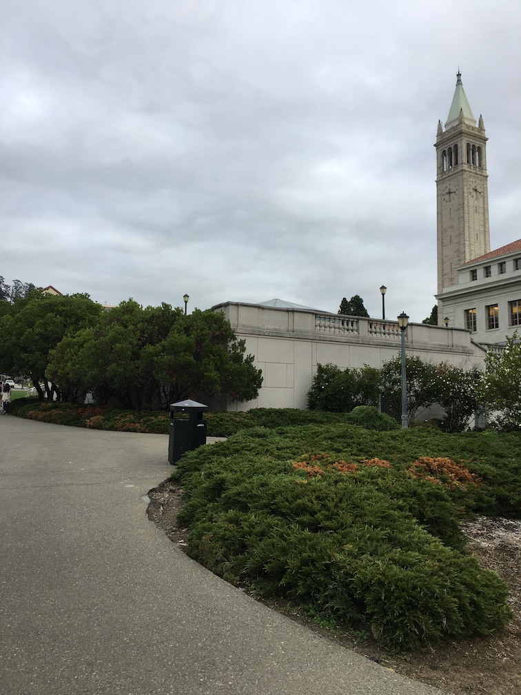
Campanile from Memorial Glade

Summary

In this second part, I learned a lot about automatic feature extraction. I really like the idea of being able to make better mosaics with less manual work.

The most interesting thing I learned is how we can detect interesting features by finding Harris corners. The math behind finding Harris corners and the fact that it works so well is pretty mind-blowing.