In this project, we build beautiful, wide-reaching panoramas composed from multiple source images warped together by homographies (pixel correspondences).
Source Digitized Images
I used my Nexus 6 smartphone camera to take beautiful, wide shots, with custom settings. Particularly, shots from far distances produce effectively planar images, which can be used for panorama reconstructions.
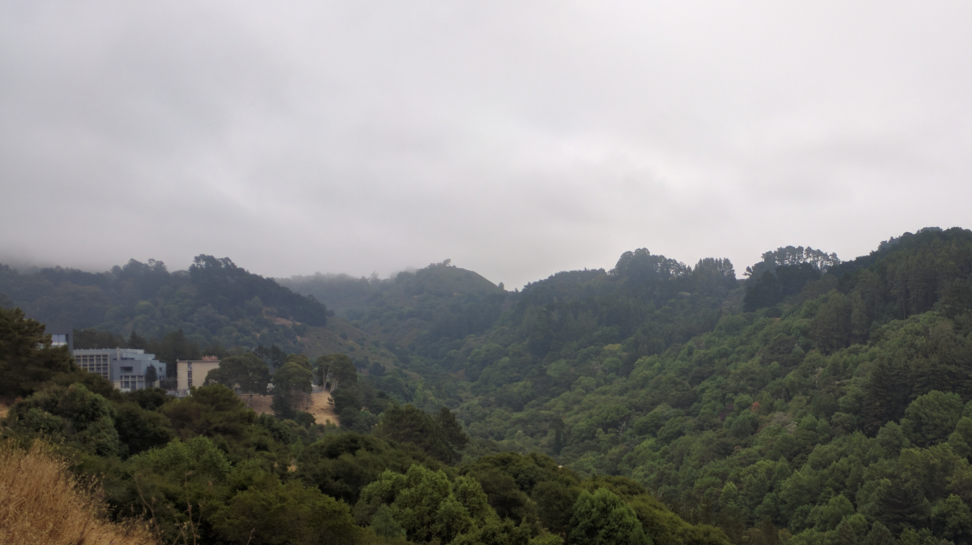
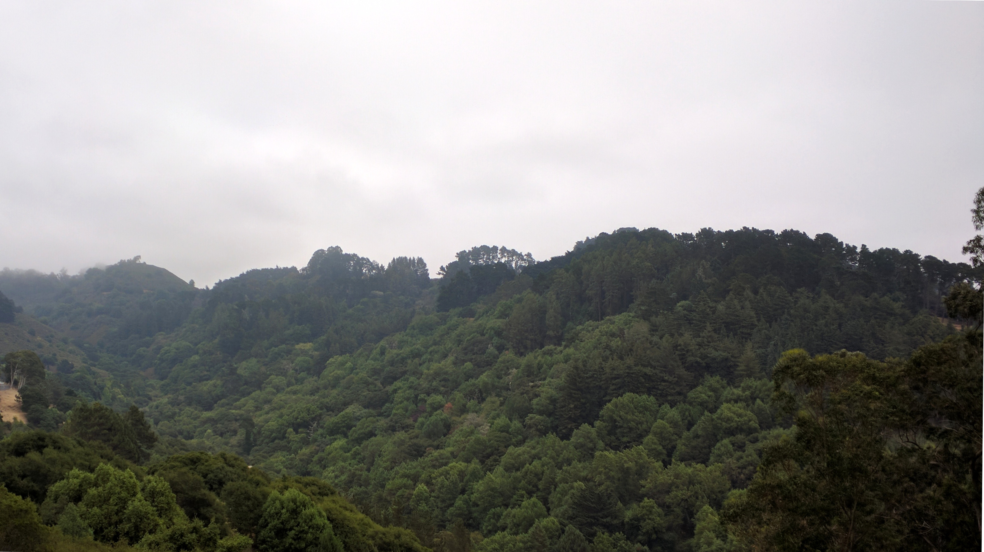
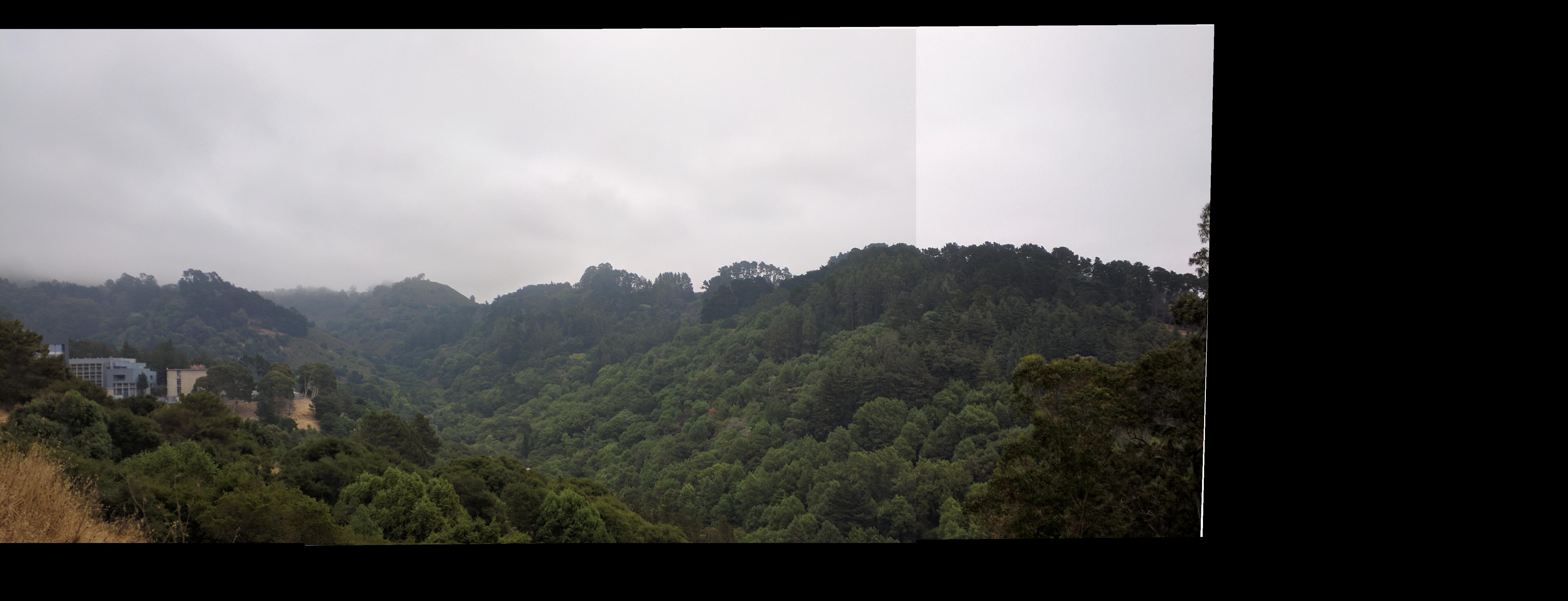
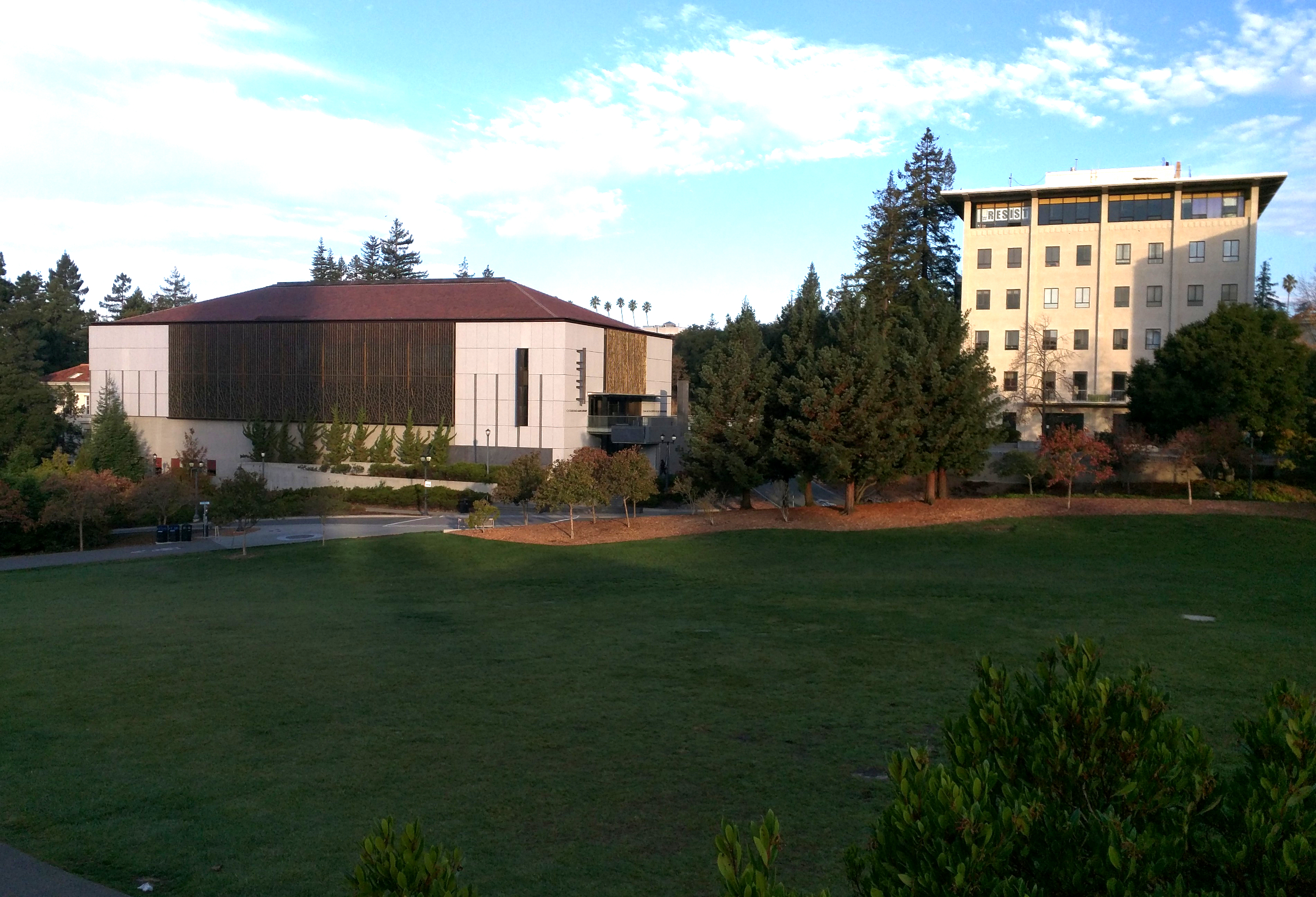
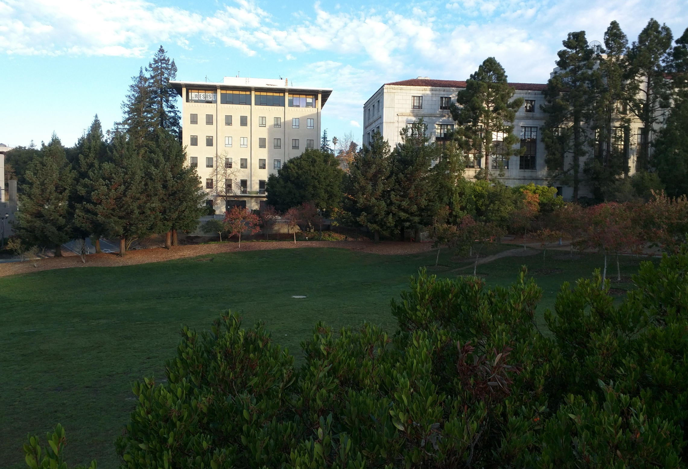
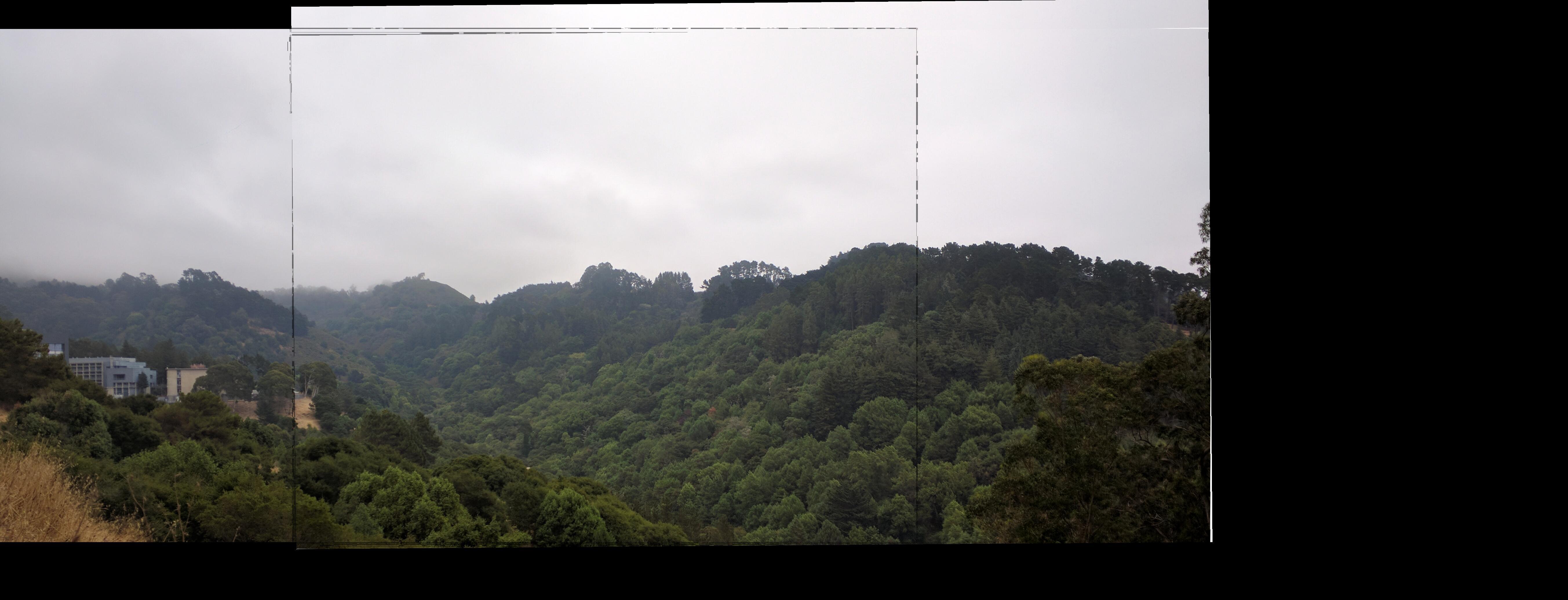
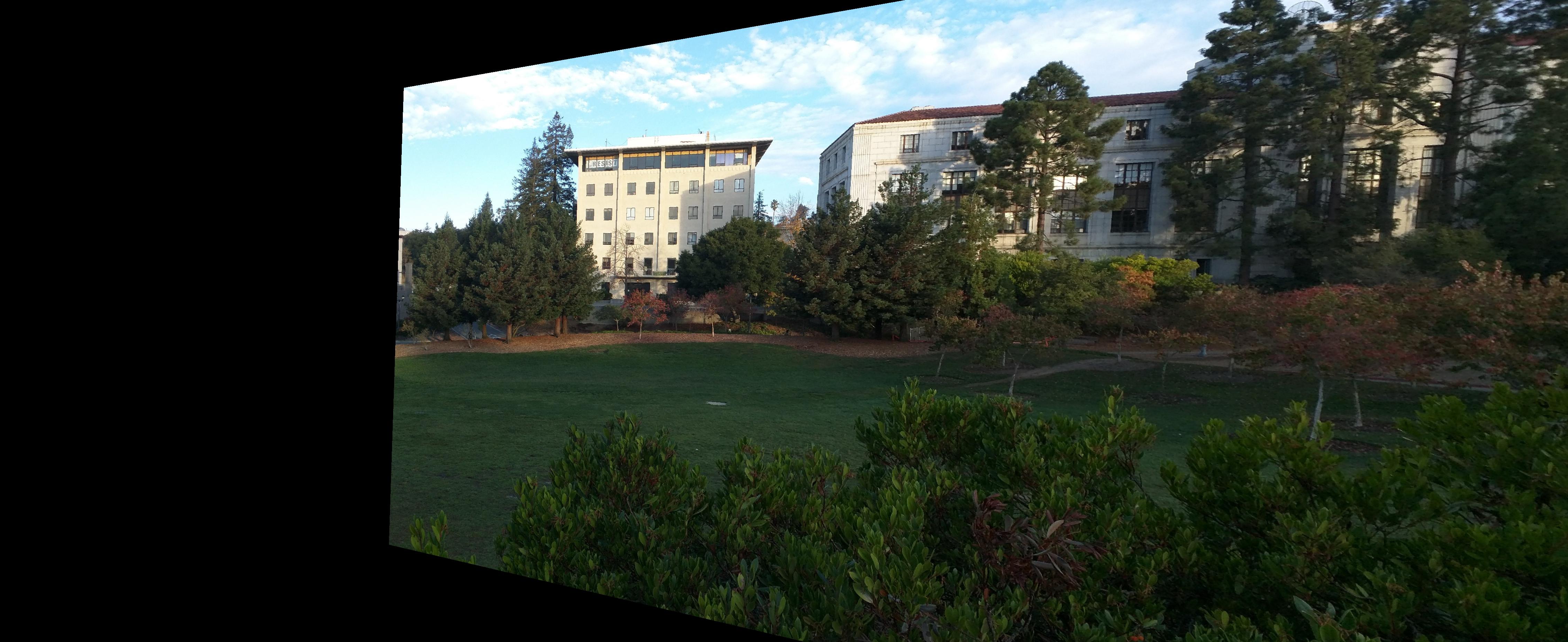
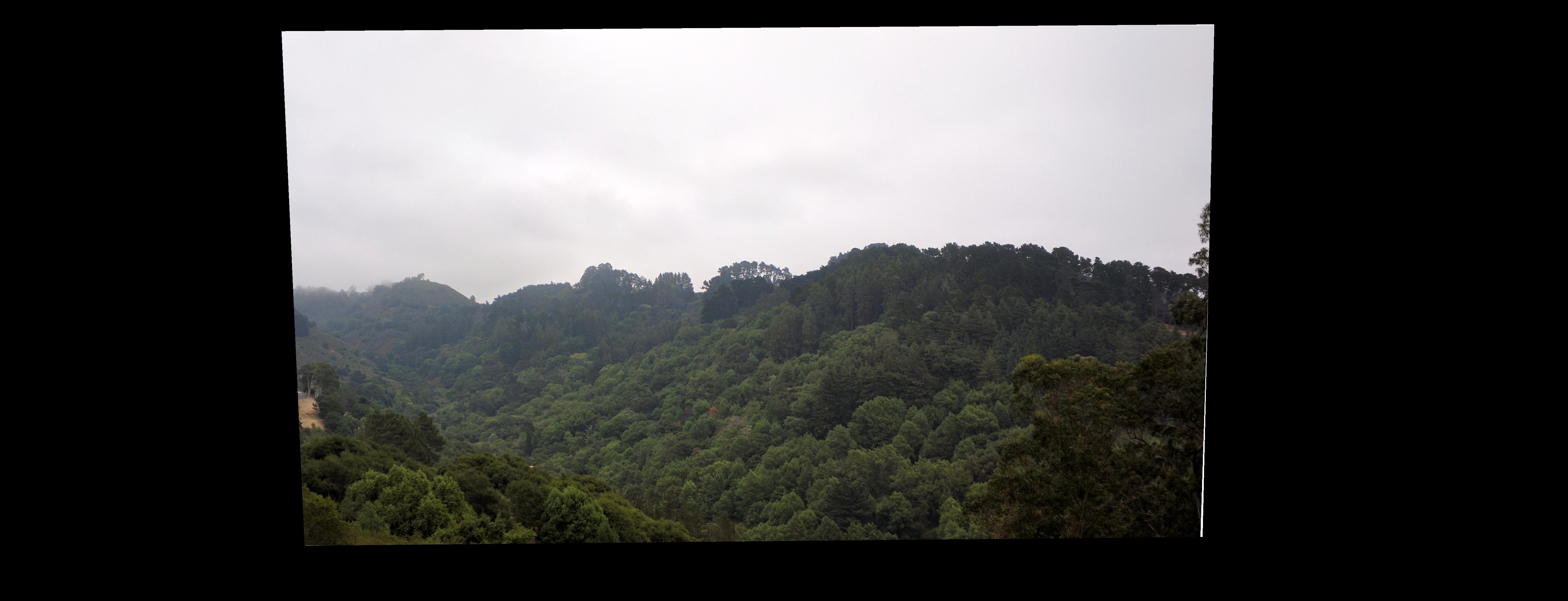
Right off the path of the Big C, looking east towards the forest outside Lawrence Lab (72 dpi, f/2, 1/154s, ISO-40, 4mm)
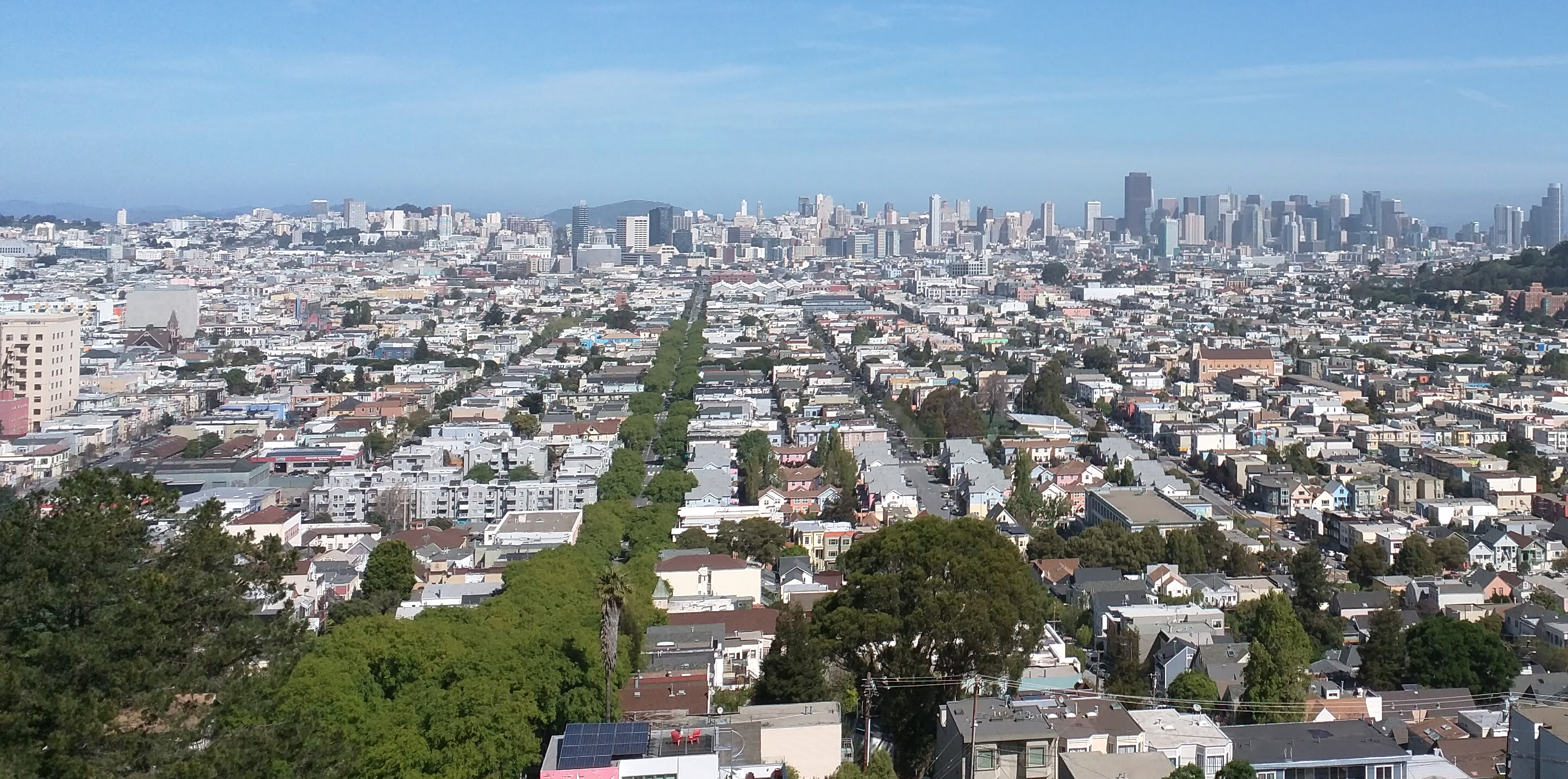
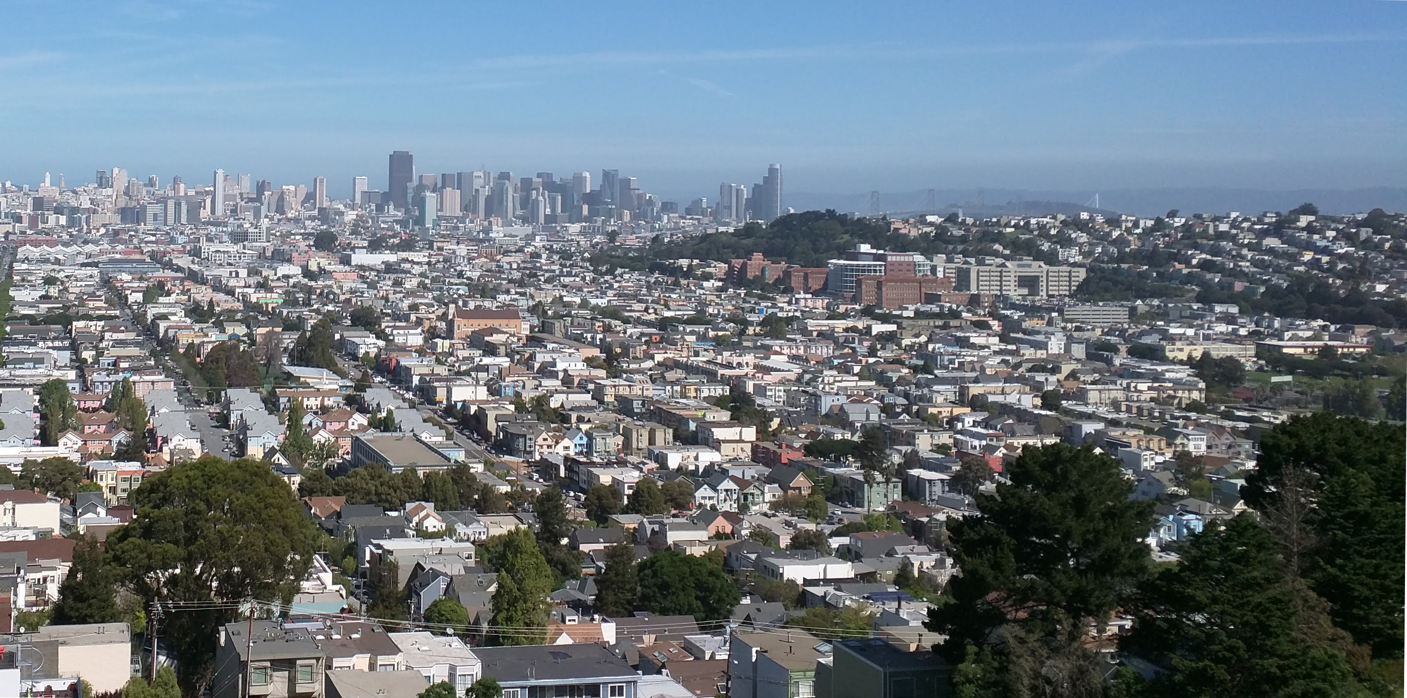
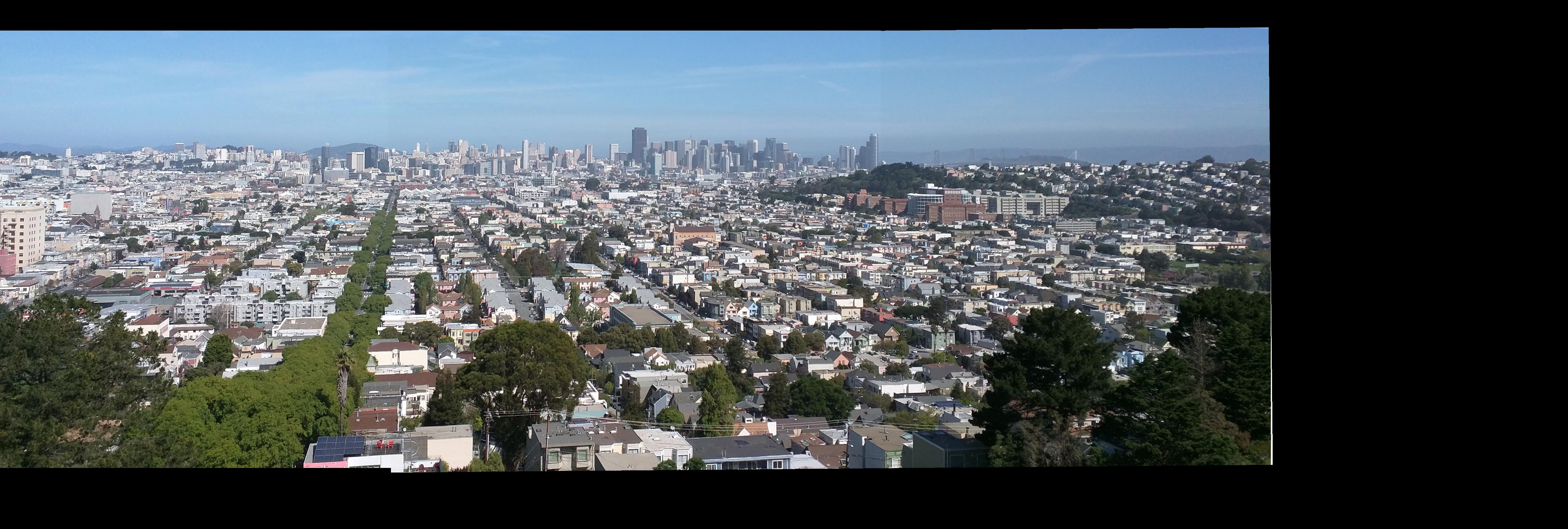
Downtown San Francisco, viewed from Bernal Heights (72 dpi, f/2, 1/2084s, ISO-40, 4mm)
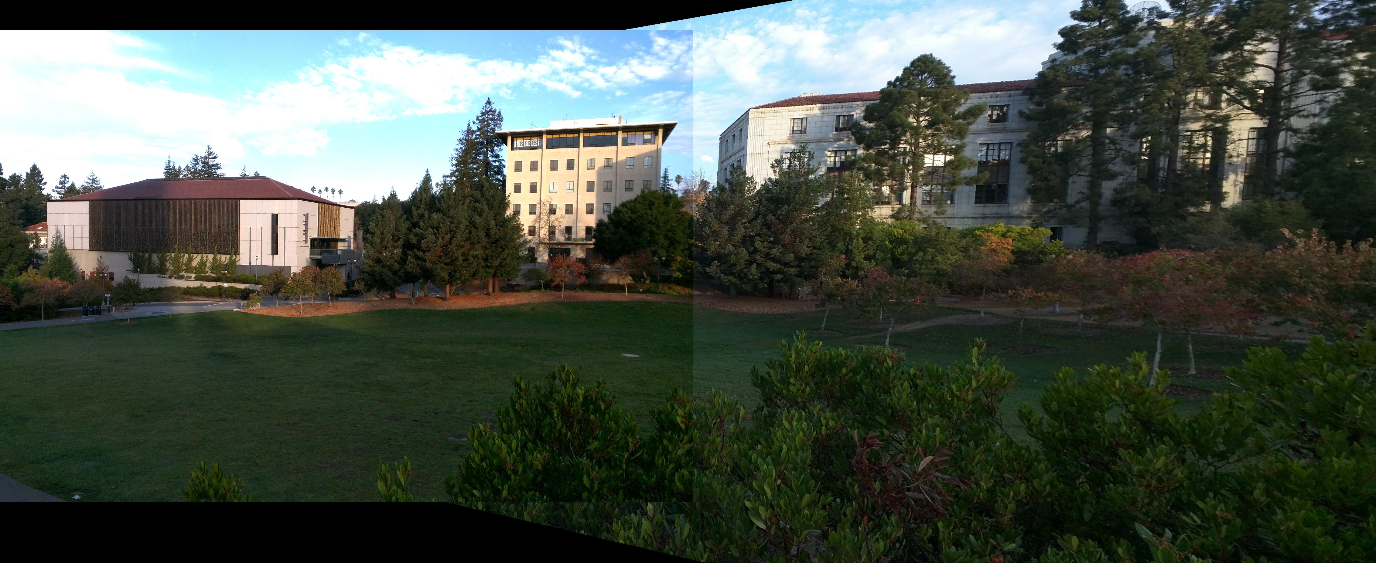
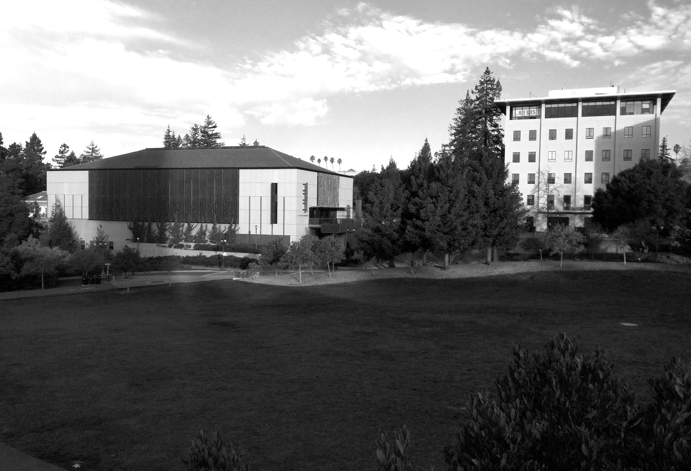
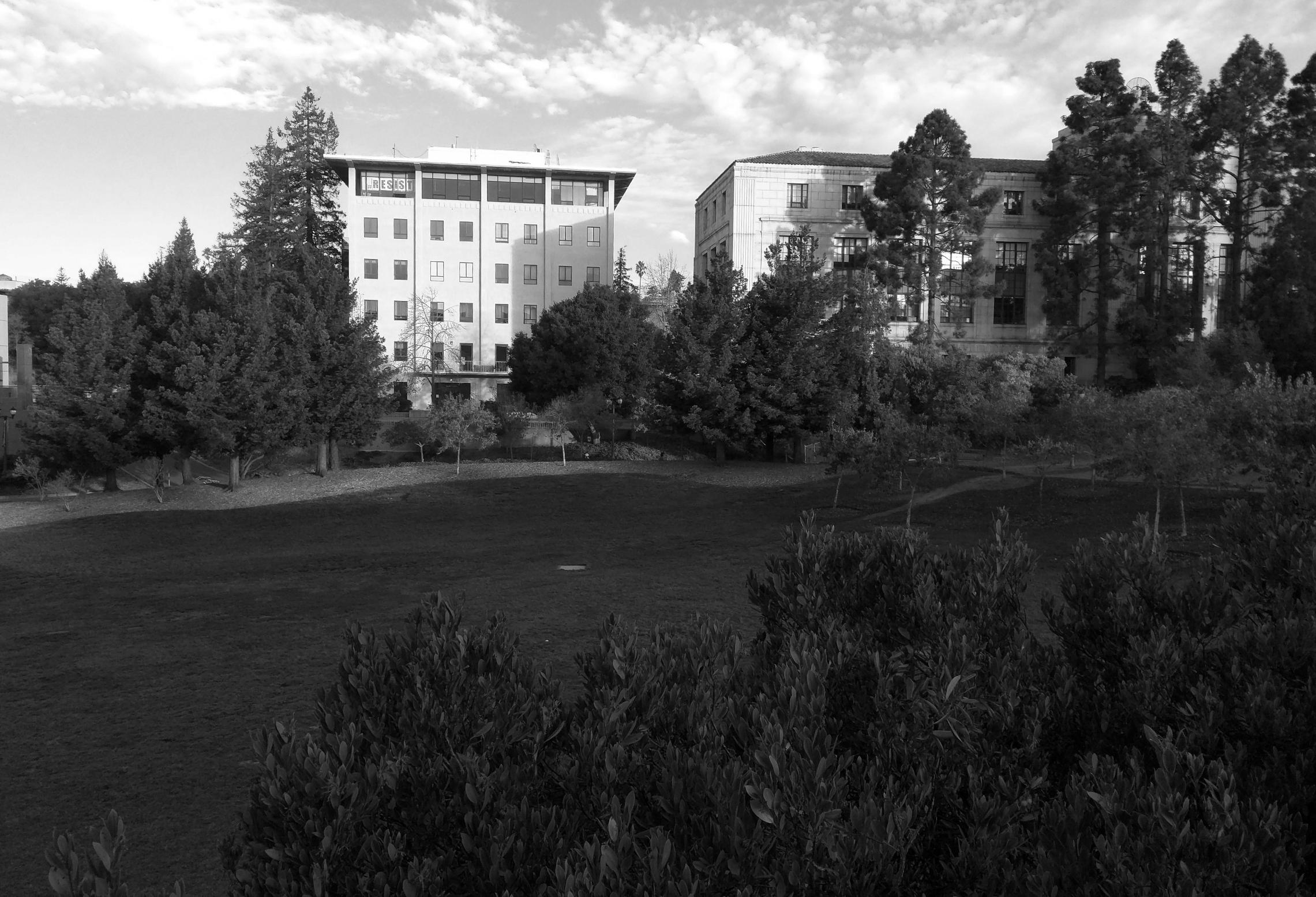
From Doe Library, overlooking the Memorial Glade in the early morning (72 dpi, f/2, 1/769s, ISO-40, 4mm) (new for part B)
Recovering Homographies
As seen in my accompanying source code, we set up the equations and solve for the homography constants $[a, ..., h]$,
$ ax + by + c = wx' $
$ dx + ey + f = wy' $
$ gx + hy + i = w, i = 1 $
$ ... $
$ a(...) + ... + h(...) = ... $
This is a least squares problem which is fully determined (i.e. uniquely solvable) by a certain $n$ correspondences, which produces $2n$ equations, one each for the x and y dimensions. When this problem is overdetermined, solve the equation as follows, where A and B are the hand-determined correspondences.
$AH \approx B \rightarrow H \approx minarg_H \vert \vert AH - B \vert \vert^2_2 $
Linear Blending, Final Panorama (Manual)
To merge the images together, I copied the left and right images onto two canvases. Then, I warped the right image to its correct place.
I merged the images together using a linear (additive) alpha mask, seen in my code.
rgb2gray
To determine Harris corners later, I converted RGB images to grayscale, using the transformation for an image $I$:
$ gray = 0.587 * I.r + 0.299 * I.g + 0.114 * I.b $
Rectifiying/Warping Images (Forgot in Part A)
Here are examples of warp flat images into their correct "position" using homography transformations.
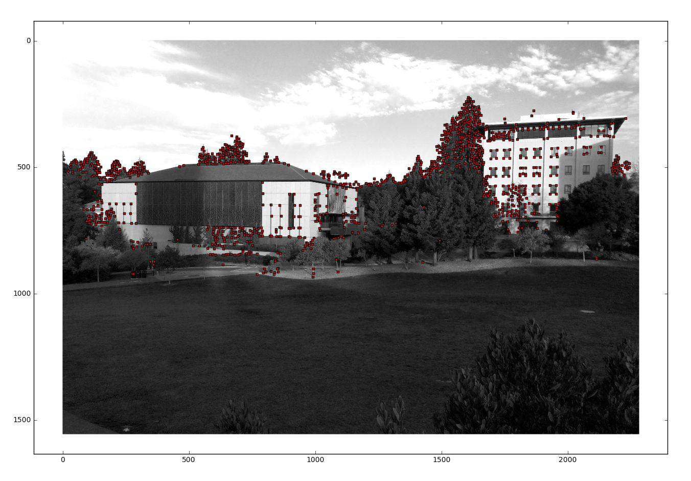
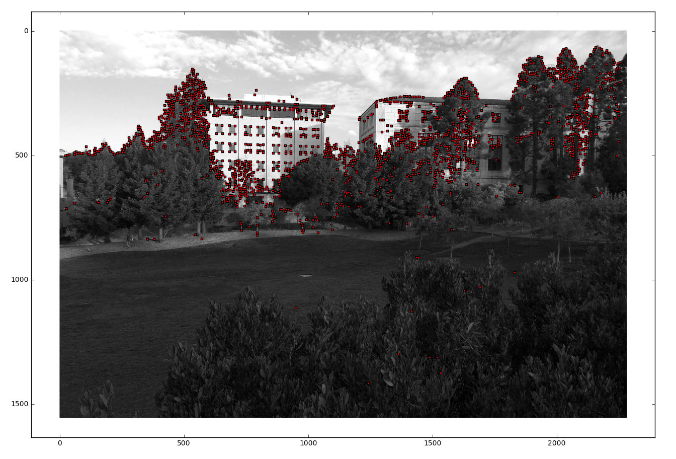
Detecting Harris Corners
I used the Harris corners source code to extract corners from the images. Intuitively, these corners are determined by the gradients across both the x and y directions.
Extracting Feature Descriptors
A Gaussian stack can be used to extract a zoomed-out, blurred feature descriptor which is more invariant to intensity and contrast shifts. I used a Gaussian pyramid and then sampled either a 9x9 (Tilden, SF) or 13x13 (Doe) window, which is flattened into a 81x1 or 169x1 vector.
Left: The pixel neighborhood around an image corner; Right: its extracted feature, grayscaled and normalized.
Matching Feature Descriptors
I used the source code to quickly compute pairwise SSD metrics between feature descriptors. According to the paper, ideally, a true matching, as opposed to a coincidental one, is such that
$ f_{1NN} \leq c * f_{2NN} $ given 1NN, the best match, and 2NN, the second-best match, and $c$ is an empirically determined constant.
In practice, I used $c$ values of 0.4 for SF and Tilden and 0.666 for the Doe panorama. Lower values of c enforce much stricter matches, but could constrain the problem too tightly in a kind of overfitting. Likewise, higher values of c increase the availability of finding both good and bad matches, but increase the number of RANSAC iterations and reliance on a robust algorithm, as well as the probability of catastrophic failure.
RANSAC Homography and Final Panorama
I used RANSAC, the coolest algorithm, to compute a robust homography estimate. It works by computing sample homographies between random sets of four correspondences, finding the homography which computes the greatest set of inliers, and then recomputing the entire homography on all of the inliers.