CS 194-26: Project 6
[Auto]Stitching Photo Mosaics
Part A: Image Warping and Mosaicing
Ellen Hong
Overview
In this project, we explore the applications of homographies in image warping and creating photo mosaics.
Image Warping
We demonstrate the results of warping images of the same scene as looked at from different perspectives. In order to create this effect, we apply a homographic transformation on the feature points from one image to another. The homography H is found by solving the following least-squares equation, where (xn, yn) is a feature point on one image, and (xn', yn') is the corresponding feature point on the other image.
Here are some examples of warped images:
 Poster, side perspective
|
 Poster, front perspective
|
 Side perspective poster, warped to front perspective
|
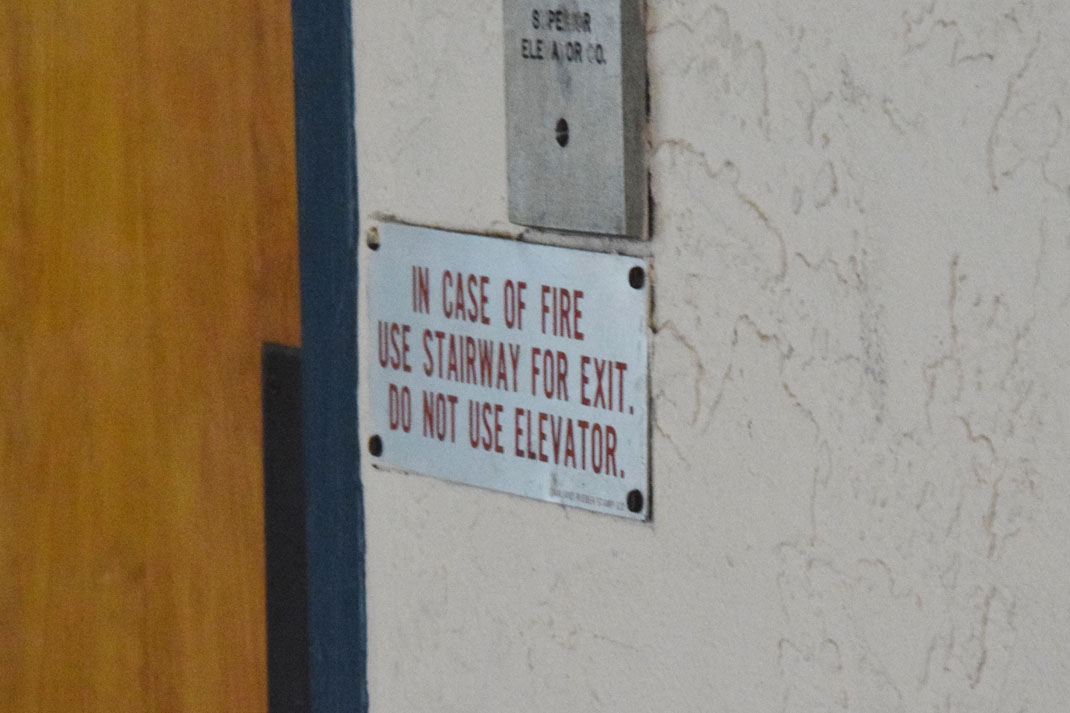 Elevator sign, side perspective
|
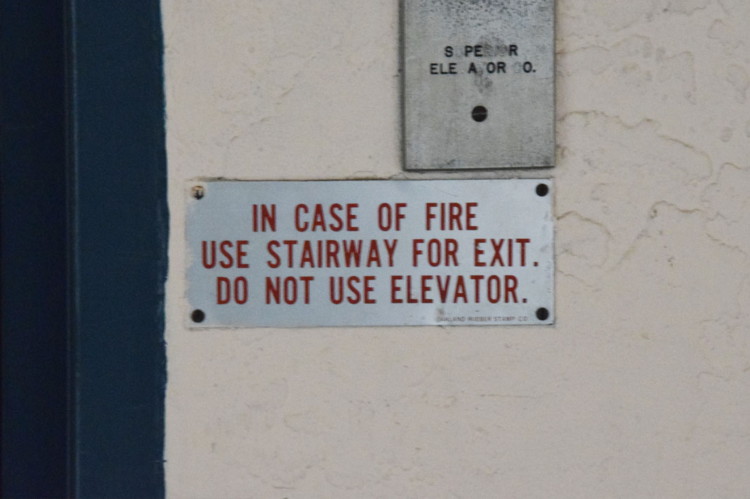 Elevator sign, front perspective
|
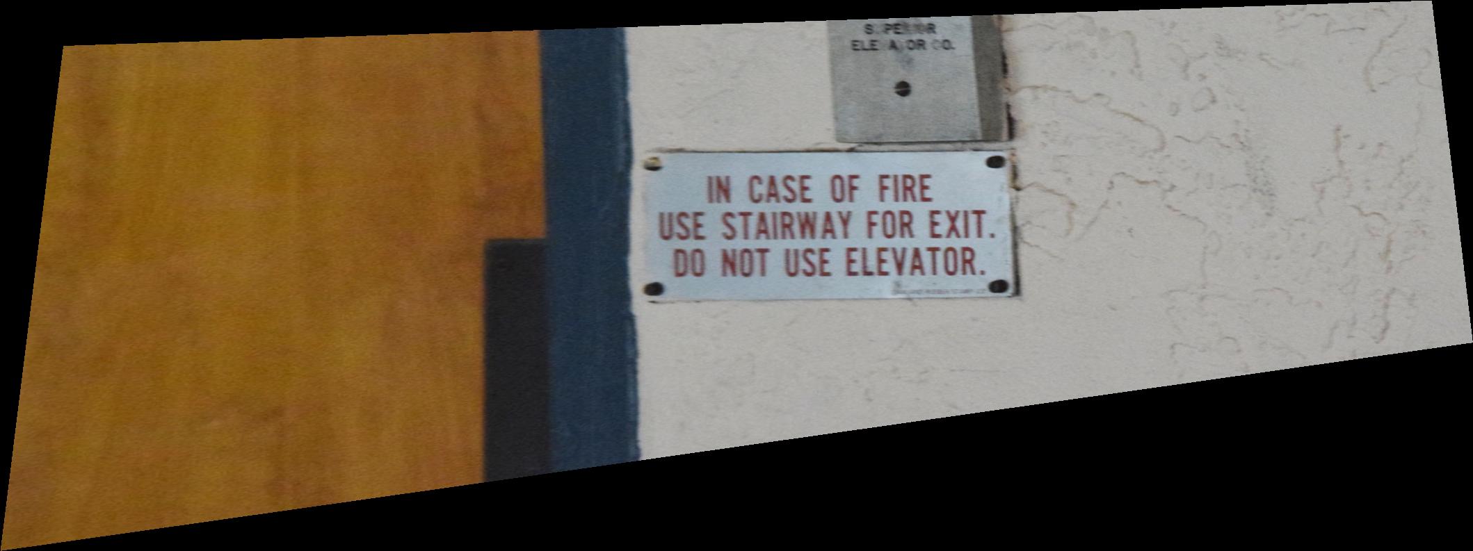 Side perspective elevator sign, warped to front perspective
|
A not-as-successful result, due to the 3-D nature of the numbers:
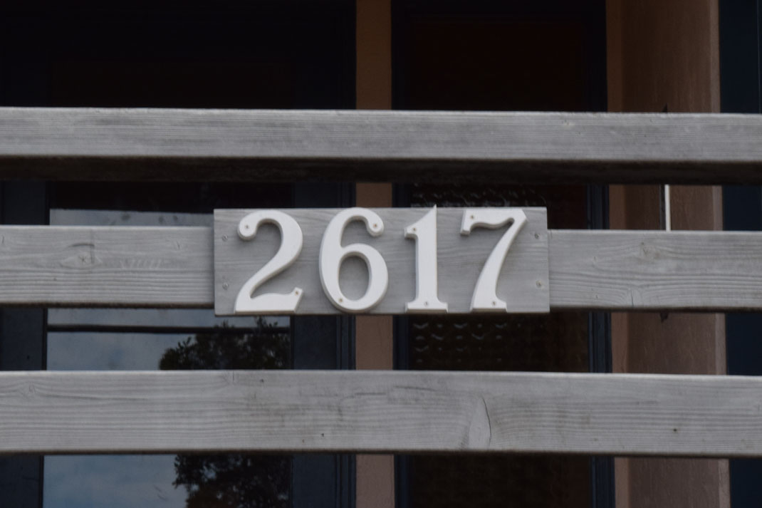 Building number, side perspective
|
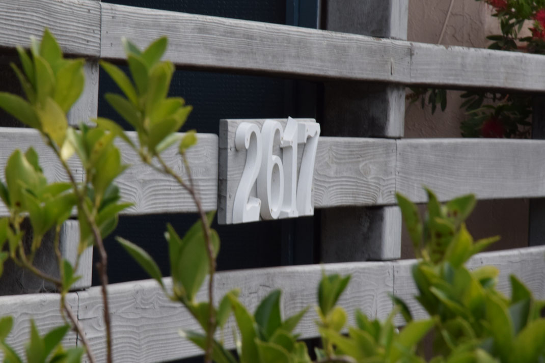 Building number, front perspective
|
 Side perspective building number, warped to front perspective
|
Image Rectification
We can also use the same homographic transformation to rectify images, i.e. change the perspective of an image by manually defining the output feature points. We produce the following results:
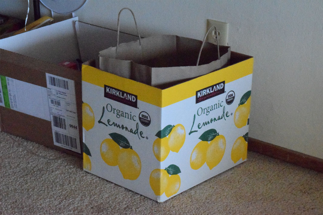 Box, side perspective
|
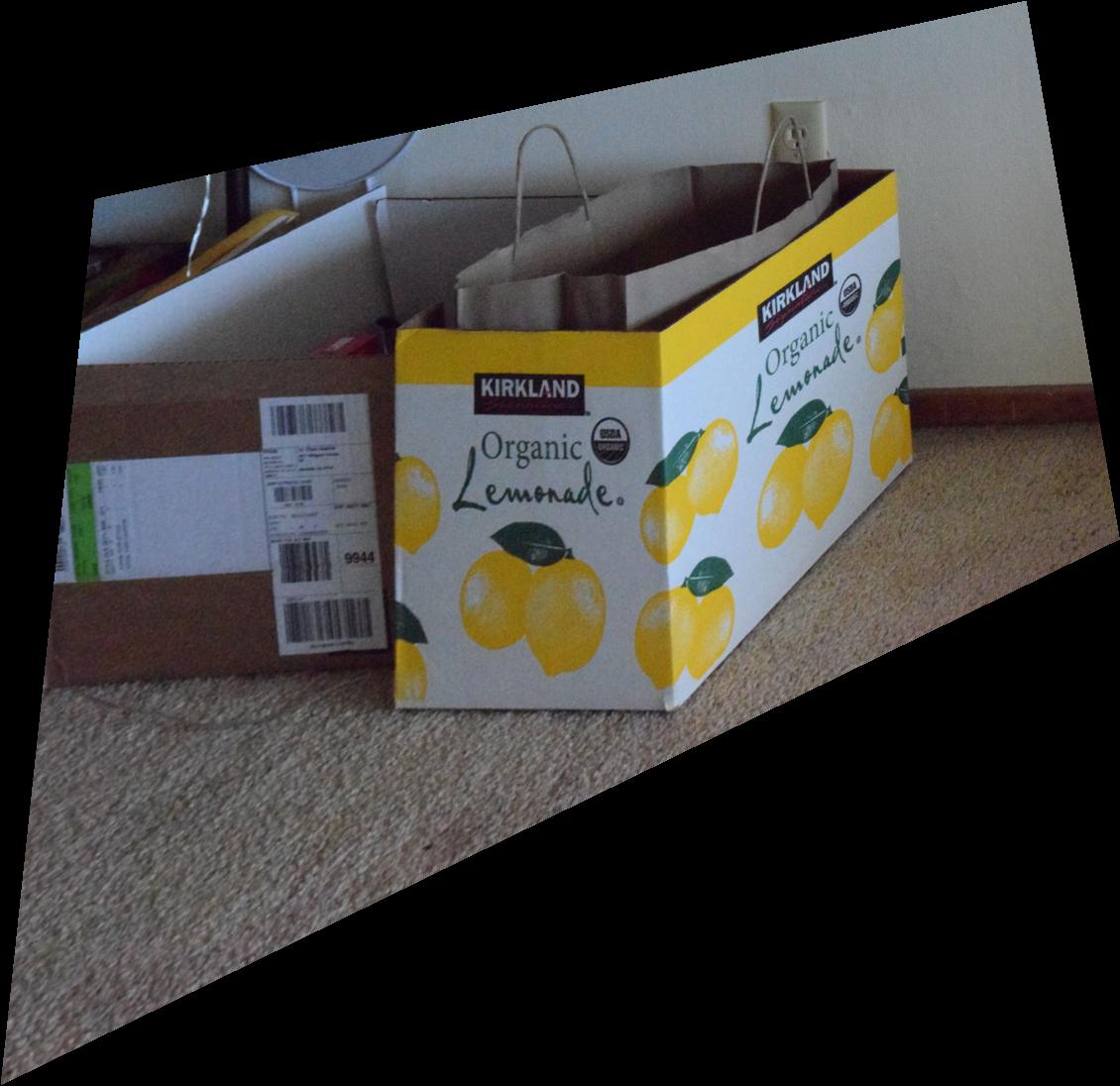 Box, warped to front perspective
|
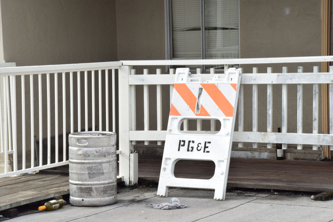 PG&E sign, side perspective
|
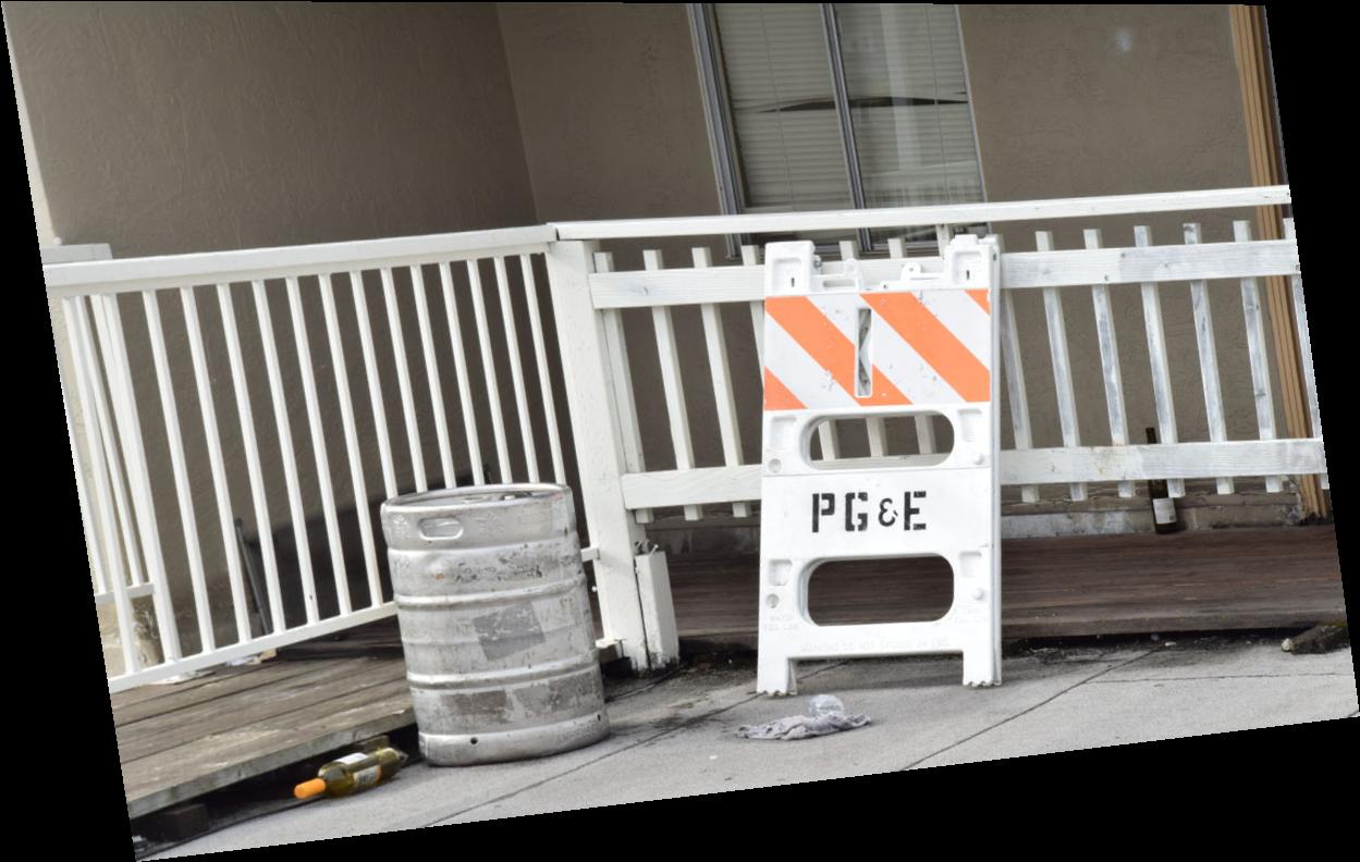 PG&E sign, warped to front perspective
|
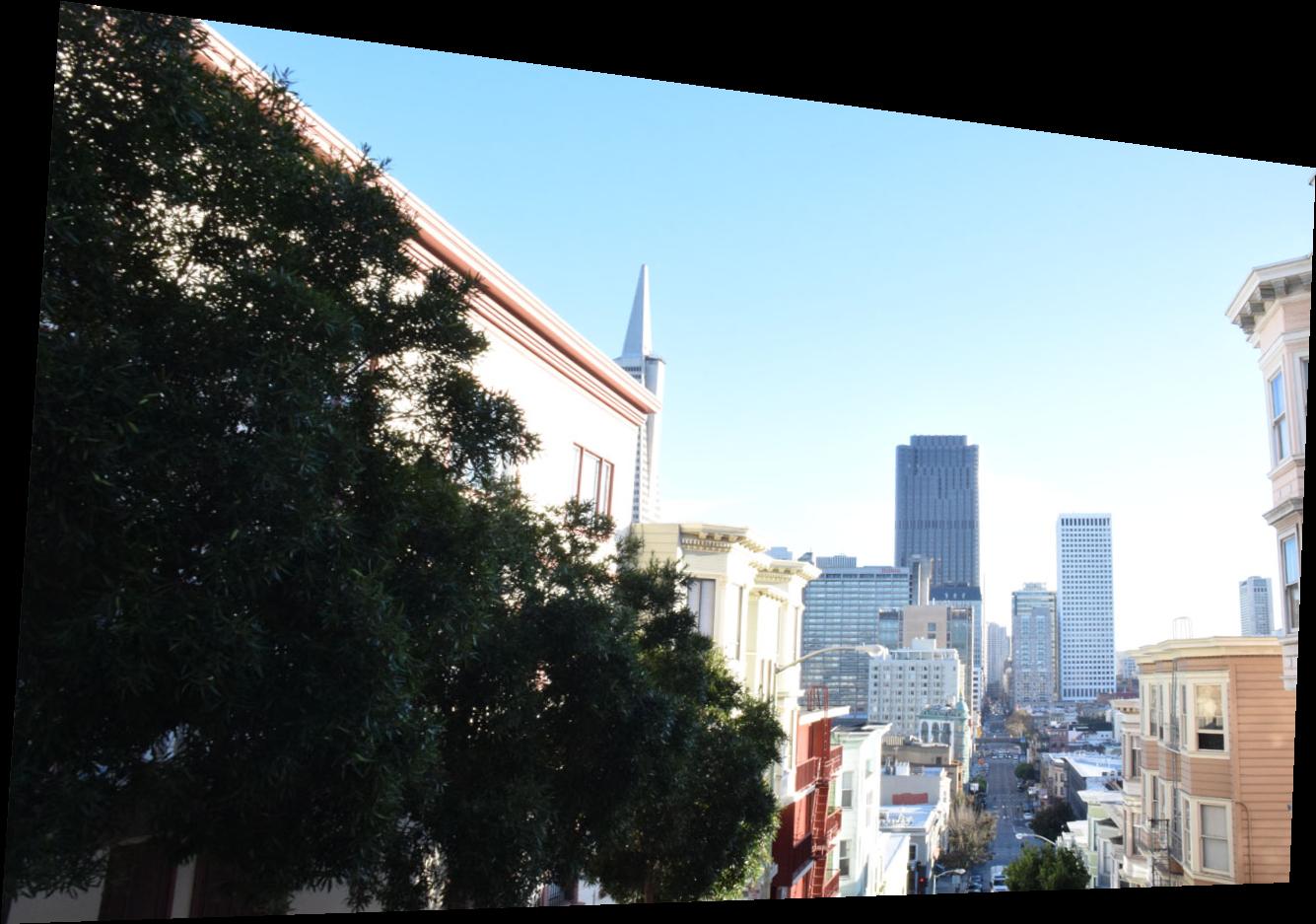
Image Mosaicing
We can now use this warping algorithm to create mosaics, by warping point correspondences from one image to another, and blending the images together via linear alpha blending. We demonstrate this technique on the following results:
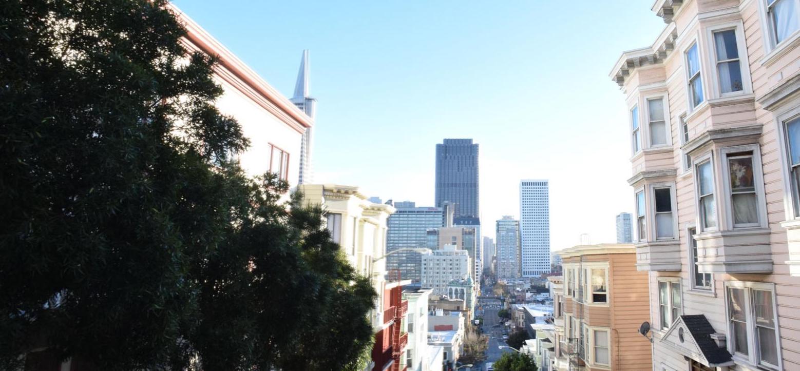
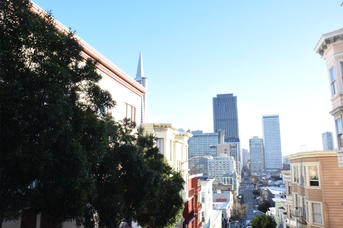 SF buildings, left view
|
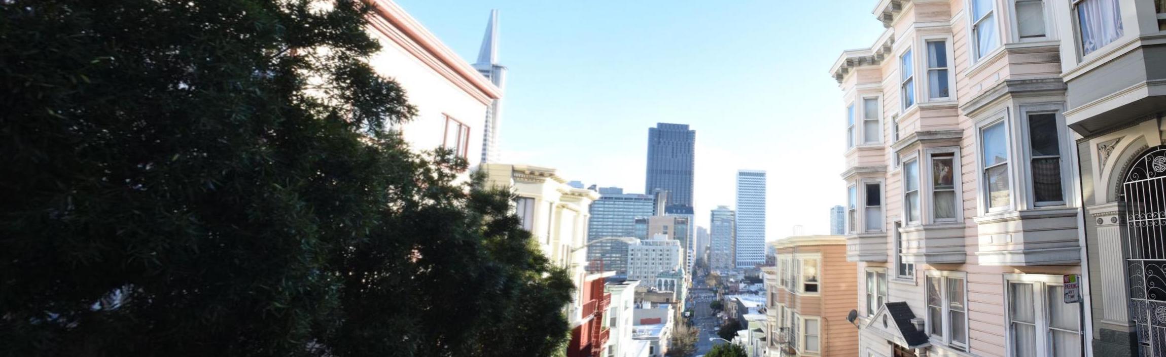
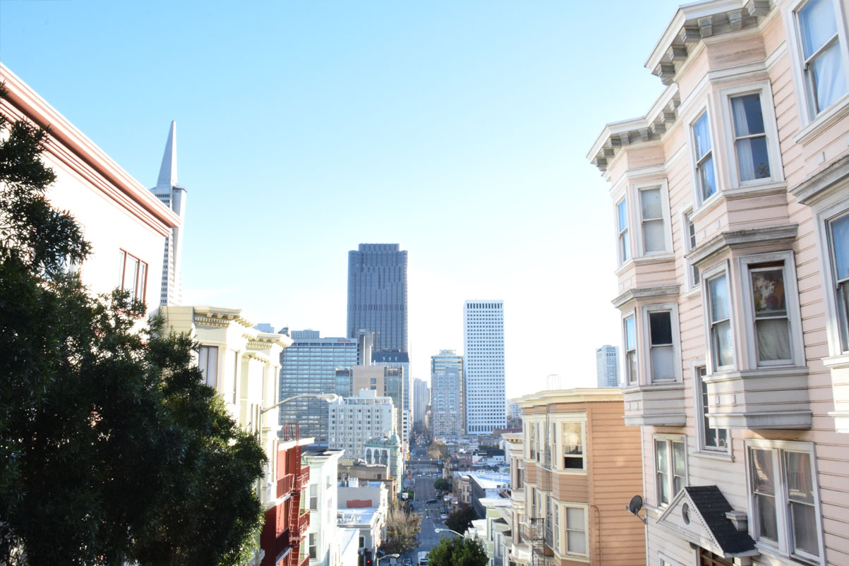 SF bulidings, front view
|
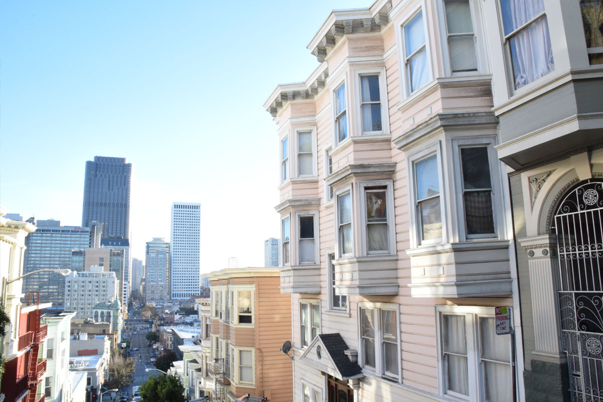 SF buildings, right view
|
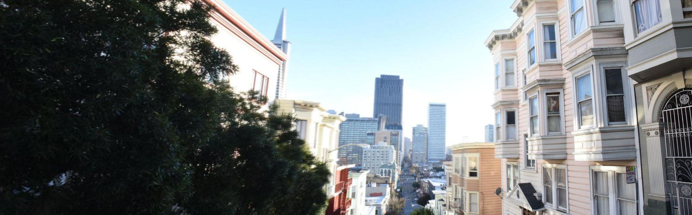 Blended mosaic, SF buildings
|
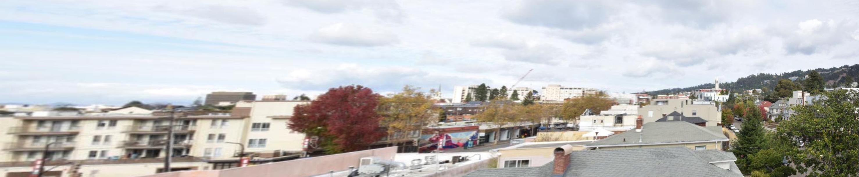
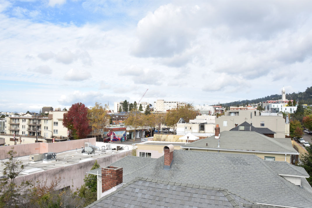 Rooftop view, left view
|
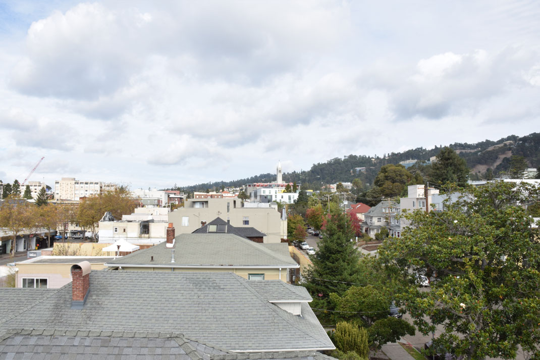 Rooftop view, front view
|
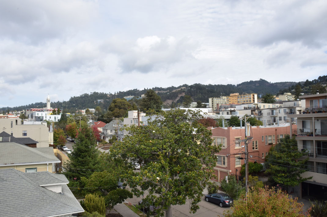 Rooftop view, right view
|
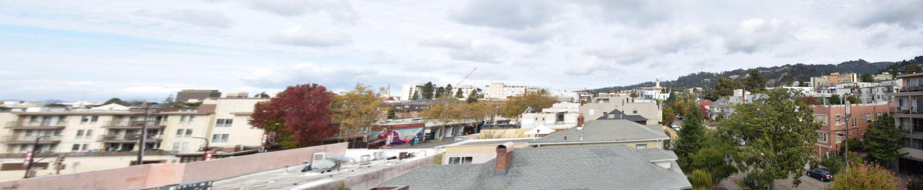 Blended mosaic, rooftop view
|
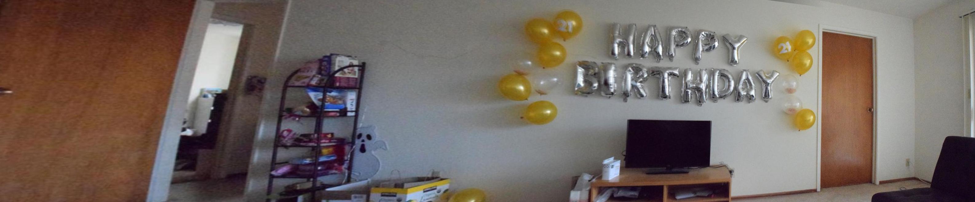
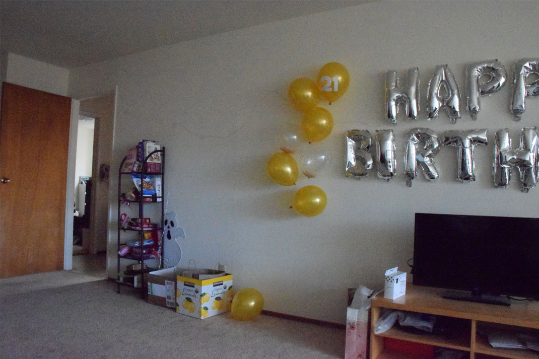 Living room, left view
|
 Living room, front view
|
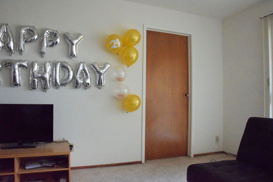 Living room, right view
|
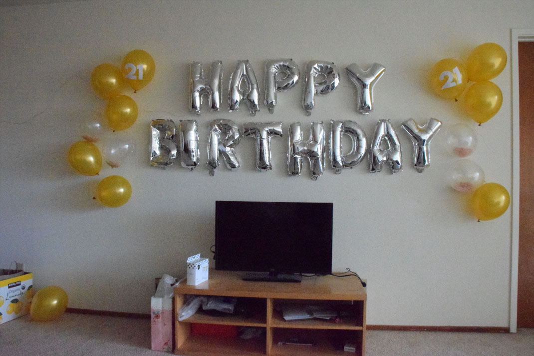
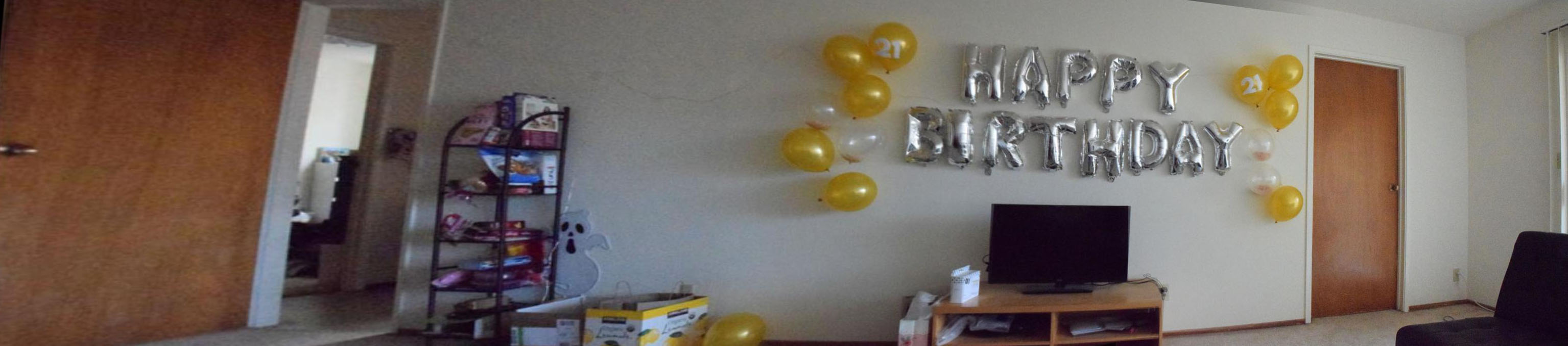 Blended mosaic, living room
|
Part B: Feature Matching for Autostitching
Overview
This part of the project allows us to automate the process of creating panoramic stitches, instead of having to hand-select correspondence points (as was done in part A). The process we use is known as MOPS, or Multi-Scale Oriented Patches. We implement the steps described in this paper.
Harris Interest Point Detector
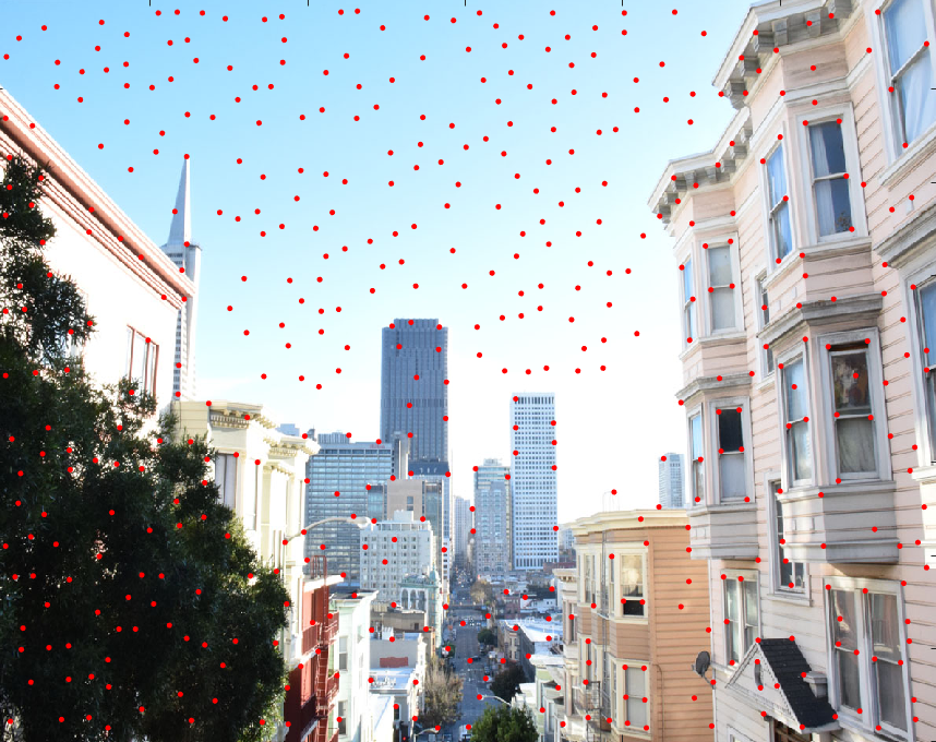
We start by using the Harris Corner Detector algorithm to find all potential corners in the image. Shown is a grayscale version of an image of SF, with Harris corners overlaid on it.
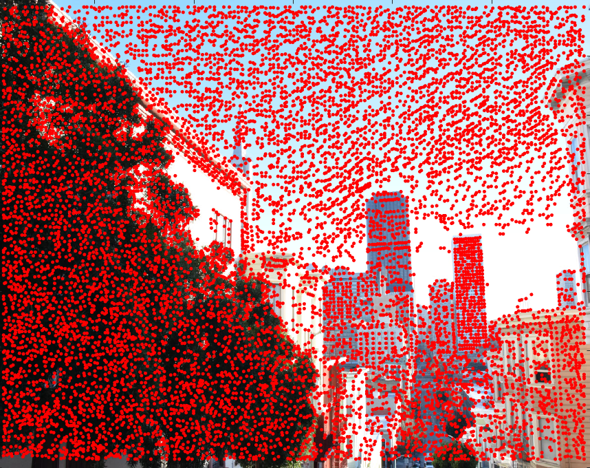 SF 1 with Harris corners
|
 SF 2 with Harris corners
|
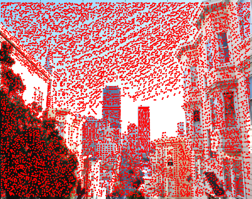
Adaptive Non-Maximal Suppression
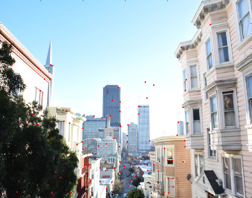
We then implement ANMS (Adaptive Non-Maximal Suppression) in order to reduce the number of features and, additionally, ensure that they are evenly distributed across each image. ANMS goes through each Harris corner point and assigns it a suppression radius. Each radius is set as the minimum radius for which one corner point is stronger than every other point within that radius. In the following results, we filter our corners down to 500 points.
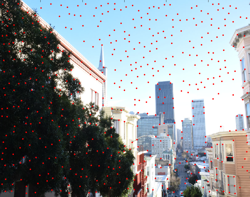 SF 1 corners, ANMS filtered
|
 SF 2 corners, ANMS filtered
|
Feature Descriptors
Now that we've identified features for each image, we need a way to describe each feature. To create a feature descriptor, we start by taking a 40x40 patch around each point. We downsample this patch to 8x8 by applying a gaussian filter and taking every 5th pixel. We apply bias/gain normalization to this patch by subtracting the mean and dividing by the standard deviation.
Feature Matching
In order to match features across images, we utilize the Lowe approach to threshold nearest neighbors. That is, for each feature in one image, we check for a match in the other image by getting its first and second nearest-neighbors, and thresholding the ratio of first-nearest-neighbor to second-nearest-neighbor. This method follows the "Russian granny" algorithm, where the idea is that if no one husband stands out from the rest, then none of them are good enough.
 SF 1 matched features
|
 SF 2 matched features
|
Random Sample Consensus
Finally, we apply RANSAC in order to secure a final set of feature points that are free of outliers. RANSAC selects 4 random points from our features points and computes a homography H. We then only keep the inliers, where the SSD of H applied to every other feature point, and their original matches, is lower than a certain threshold. Below are the results of running 5,000 iterations of RANSAC on our feature matches.
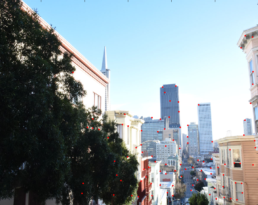 SF 1, inliers from RANSAC
|
 SF 2, inliers from RANSAC
|
We can finally use this homography from RANSAC to warp and create mosaics of these images in the same way as in part A. Below are the automatically generated warped image and mosaic of SF1 and SF2.
 SF 1, warped to SF 2
|
 mosaic, SF 1 and SF 2
|
Now, we add in SF3 to create 3-image mosaic, as was done in part A. Below is a comparison between manually and automatically stitched results:
 SF, automatically generated mosaic
|
|
SF, manually generated mosaic
|
The results look fairly similar; however, we notice that one visible misalignment in the automatic result is the ghosting we get in the Transamerica Pyramid on the left. This is because after ANMS, feature matching, and RANSAC, there was no feature point on that buliding. However in our manually generated result, I placed correspondence points on that building to ensure that the images lined up there.
We compare how our automatic stitching does on the other images from part A as well:
 Rooftop view, automatically generated mosaic
|
|
Rooftop view, manually generated mosaic
|
 Living room, automatically generated mosaic
|
|
Living room, manually generated mosaic
|
Again, we notice that the automatic results are slightly blurrier in a few areas, as compared to the manual ones. This, again, is a result of carefully choosing many good correspondence points in the manual result, points that might've been missed in the automatic stitching. All in all, however, the automatic stitching performs fairly well!
Lessons Learned
It's amazing what kinds of things a few dozen lines of code are capable of automating. I definitely learned a lot in the way of how complex yet simple it is to create image mosaics. It was rewarding to implement the automatic stitching after having to hand-select 50+ correspondence points for my detailed panoramic images. It was also cool to see how each step (from ANMS, feature matching, RANSAC) narrowed down the number of feature points more and more, into a set of points that looked closer and closer to the points I hand-selected myself in the first part of the project.