To create image mosaics, we need to do this:
H from all images to the center image with linear algebra.H to warp non-center images.
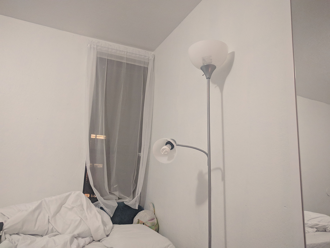
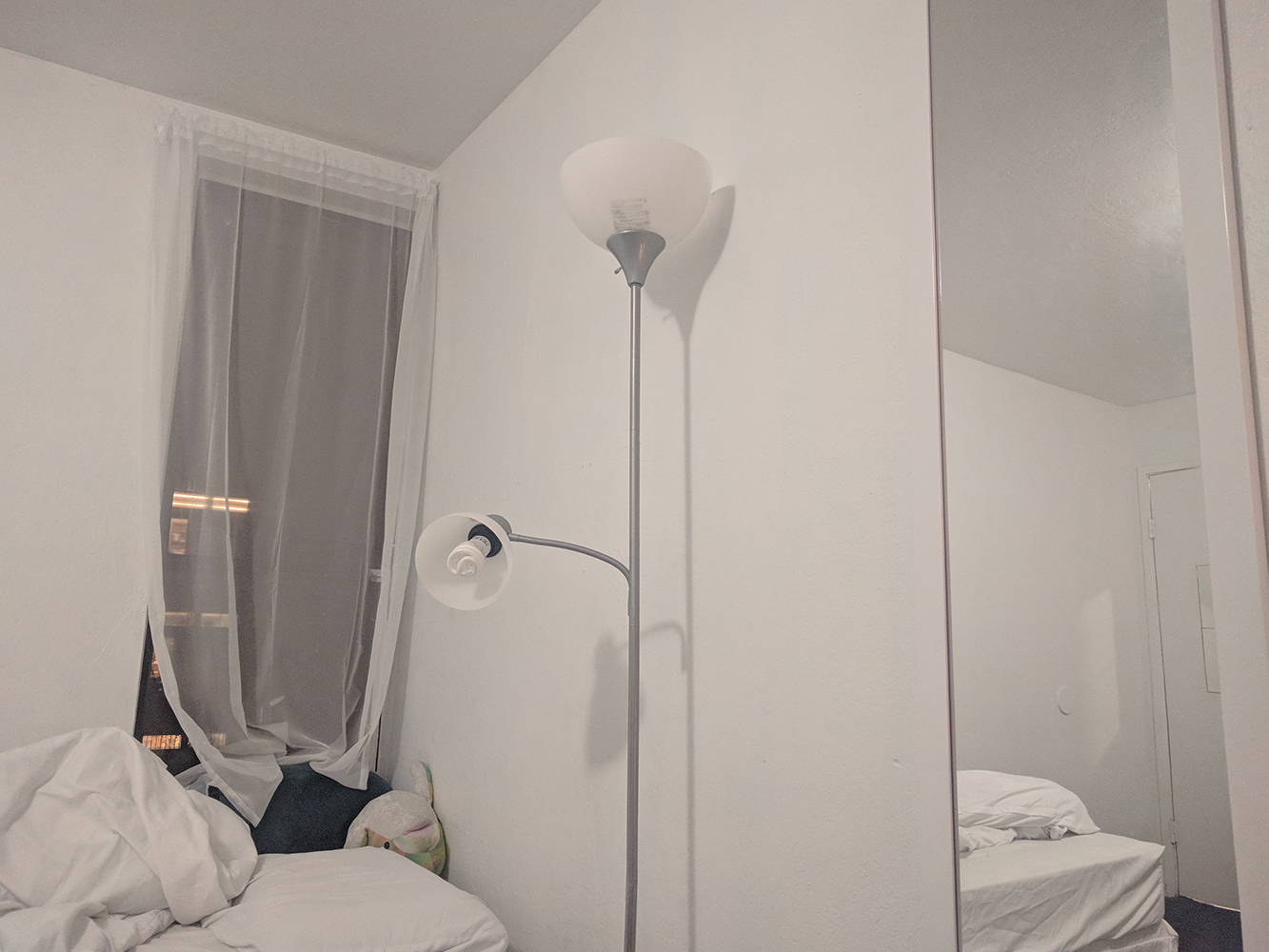
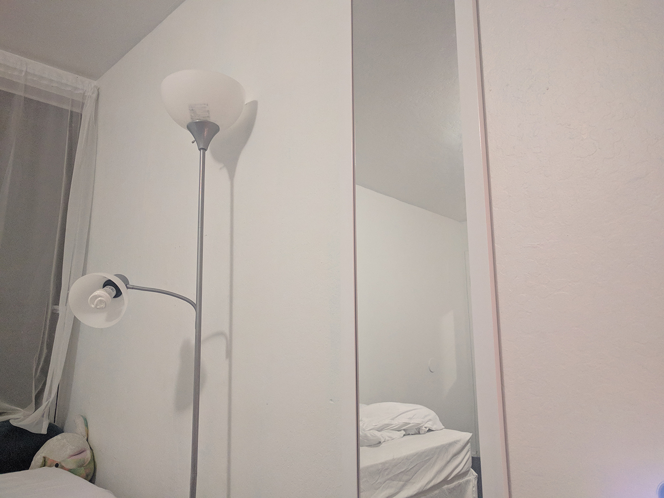
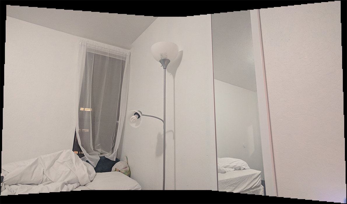
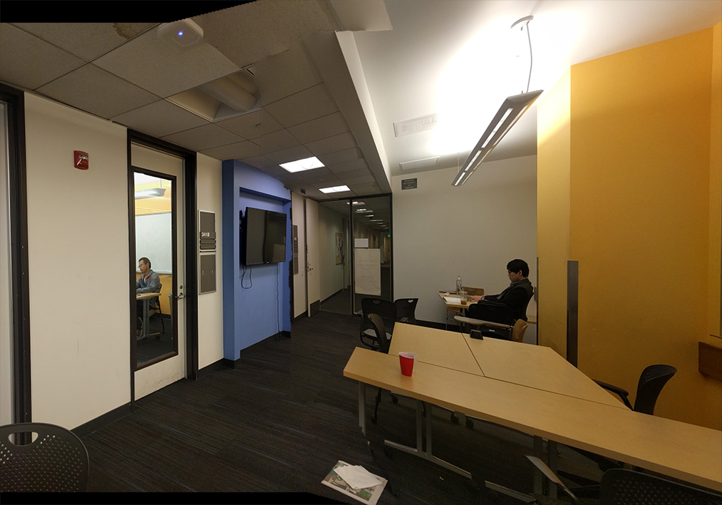
Part 1: Shooting Pictures It is important to take pictures such that there is a decent amount (40% to 70%) of overlap.


Part 2: Recover Homographies
Given the following format for homographies:
[w*x']   [a b c]   [x]
[w*y'] = [d e f] * [y]
[ w ] [g h 1] [1]x' = a*x + b*y + c - g*x*x' - h*y*x'
y' = d*x + e*y + f - g*x*y' - h*y*y'Ah = b matrix: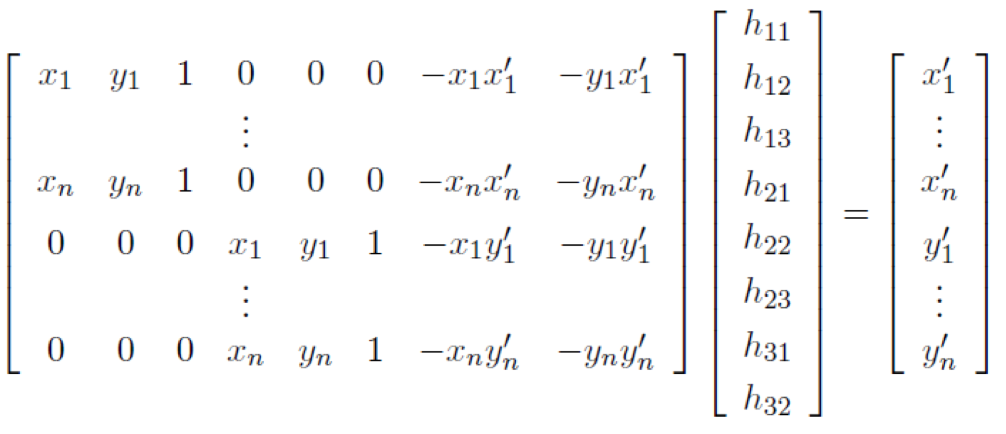
h in Ah = b with least squares, tack on a 1 at the end, and reshape into a 3 x 3 matrix. This is our homography matrix, H.After defining the correspondences by hand, we wrote a function to fine-tune them automatically with SSD over various displacements in a 10 x 10 box.
Part 3: Image Warping and Rectification
To warp images, we found the dot product between the homography H and the point we wanted to warp away from. Then we solved for w and divided the resulting x and y element-wise by w to account for it. This is an example of an inverse warp.
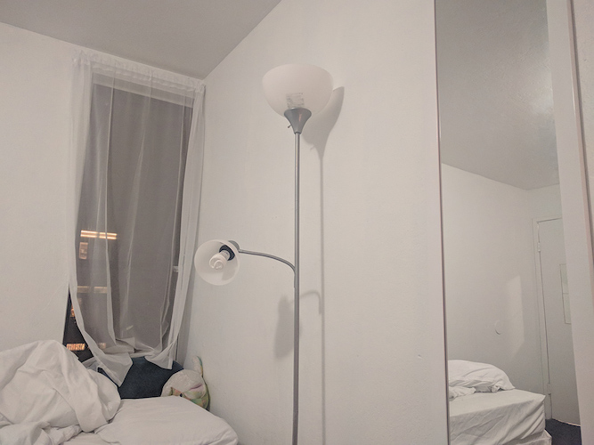
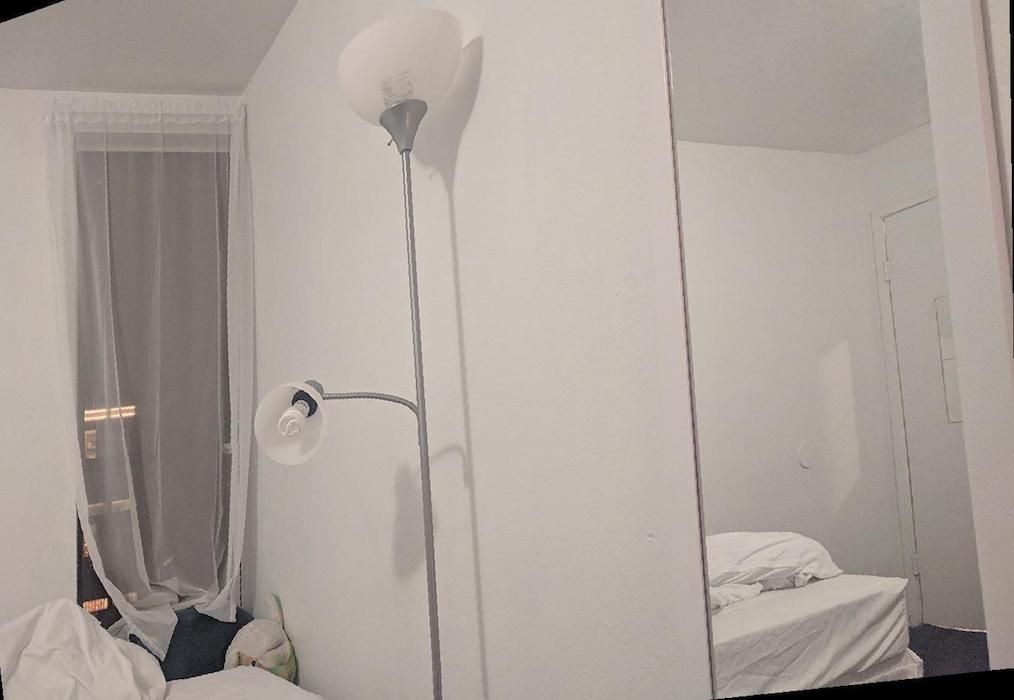
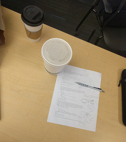
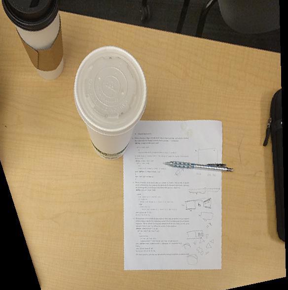
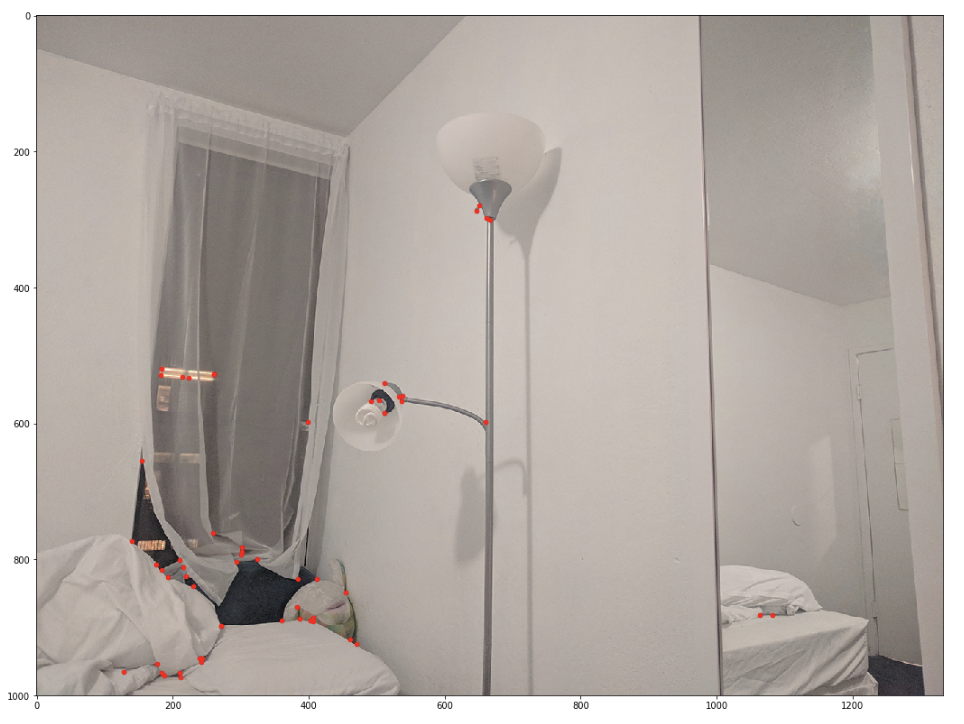
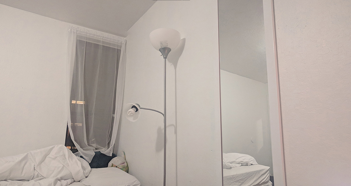
At this time, we were able to rectify images--taking a section of an image, declaring it should be a certain shape (say, a perfect rectangle, as in the window and the paper below), and warping the image to that shape. As a result, the plane is "frontal-parallel".
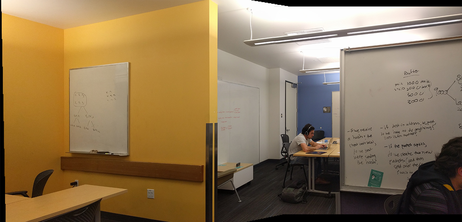
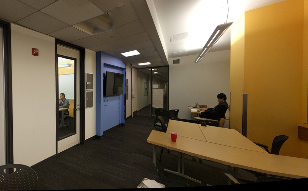
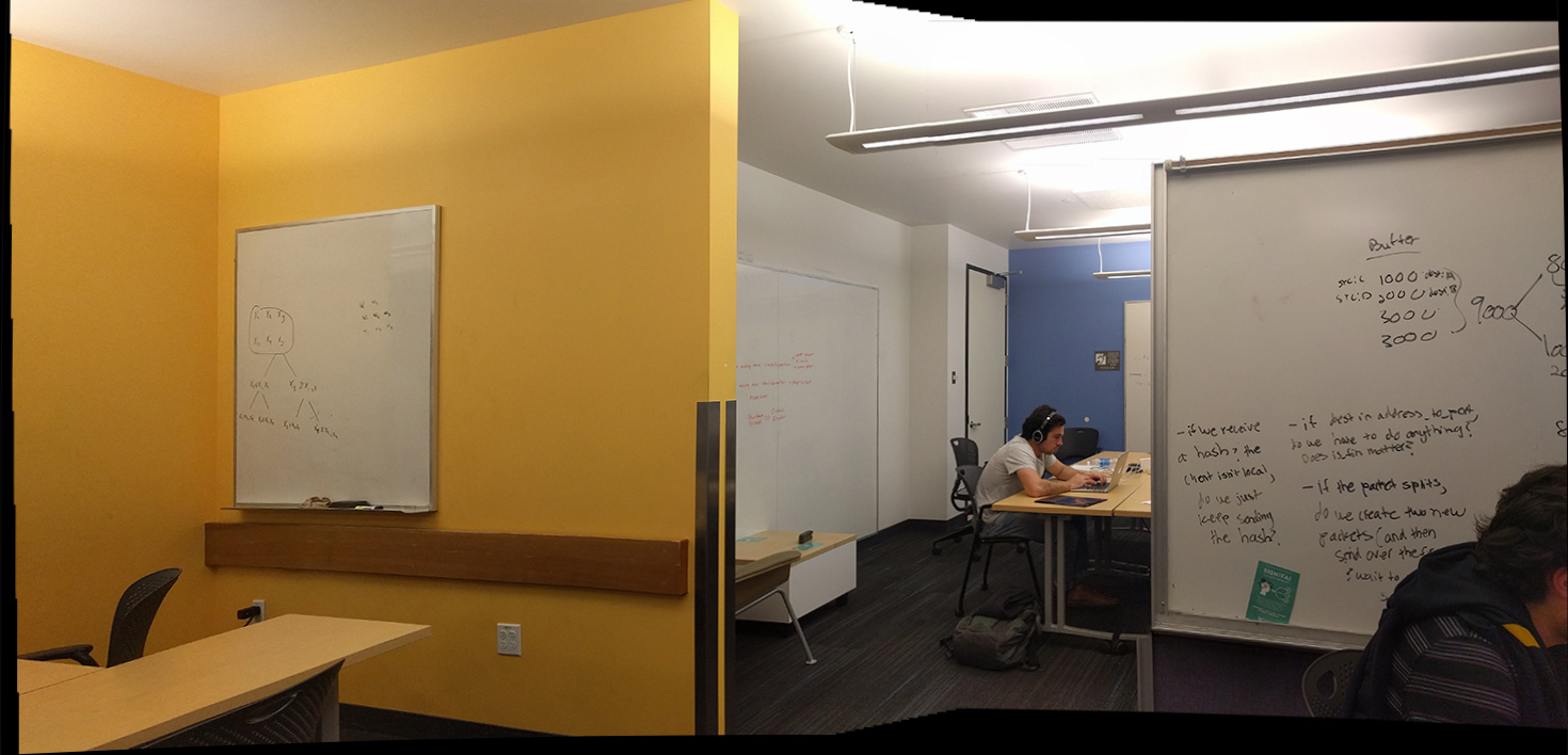
Part 4: Mosaics
Quite similar to above; this time, we took the images we shot from Part 1 that weren't in the center and warped them to the shape of the middle image. To not accidentally lose data (since scikit-image is fond of cropping off edges) we pad around the middle image with some 500 pixels each time.
Finally, we used alpha-blending with a mask to seamlessly blend images together into a mosaic.
Tell us what you've learned! Creating rectified view of single images is surprisingly simple, and is pretty cool!
To automatically select points so we don't have to manually assign them:
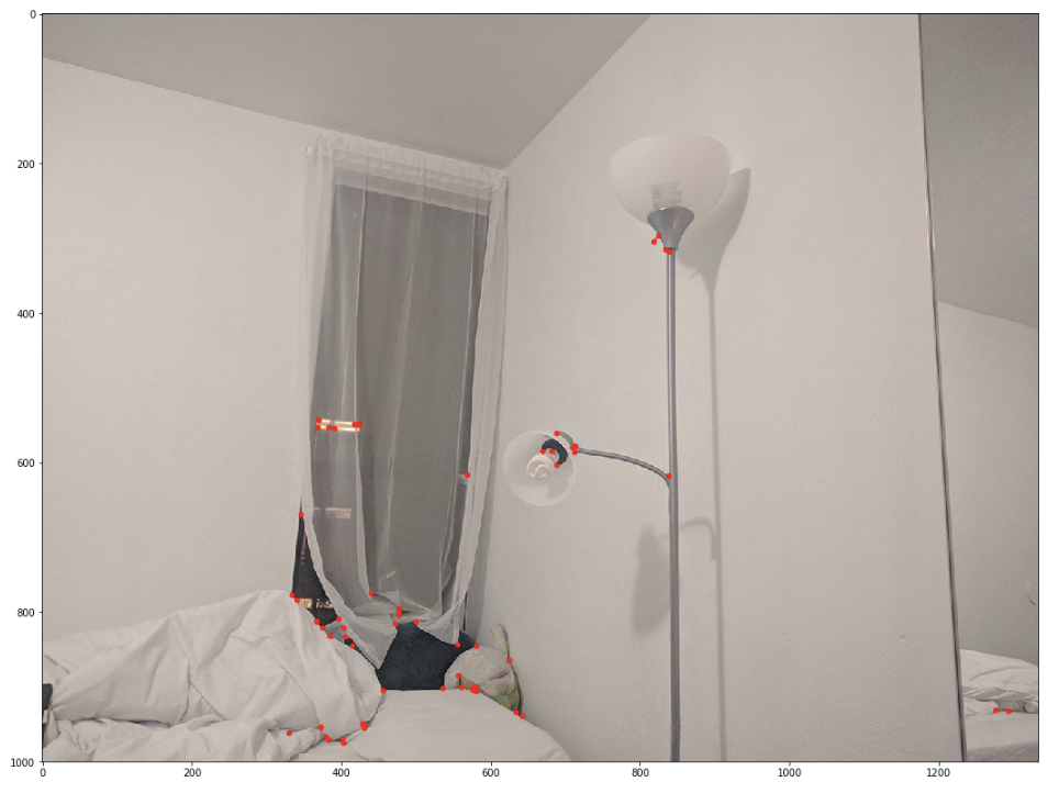
Part 1: Harris Corner Extraction We run the given code on our images, and realize pretty quickly that it gives us way too many points.
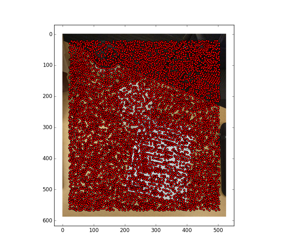
Part 2: Adaptive Non-Maximal Suppression To filter the points down, we use Adaptive Non-Maximal Suppression.
I'm going to copy and paste my description for this bit from my code here:
""" Given H (matrices of H values) and P (list of Harris corners),
for each Harris point P_I, find its suppression radius R_I, or the
smallest distance between P_I and another point P_J such that the
corner strength of P_I happens to be less than C times the corner
strength of P_J. That is, F_h(P_I) < C * F_h(P_J).

Return the first (number here) values.
"""
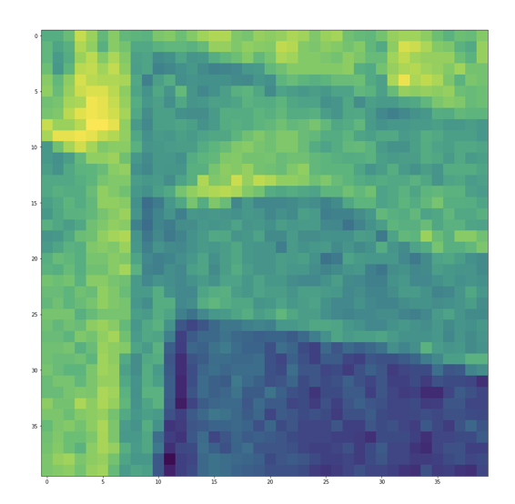
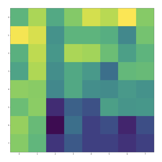
Part 3: Feature Description For each point, we took a 40x40 patch around that point, scaled it down to a 8x8 square, flattened it into a 1x64 vector, then normalized it so the mean is 0 and the SD is 1. This is so we have a simple way of mathematically identifying and comparing each point against each other, so that when we check for similarity, it's easy.
On the left is a sample 40x40 square, and on the right is the square after reducing it down to an 8x8 patch (ignore colors).
Part 4: Lowe Thresholding To discern which points should be paired with which points across both images, we used Lowe thresholding.
The SSD between each point in both images computed. For each point in img1, we look over all the points in img2-SSD'd-with-that-img1-point. If lowest SSD match has a SSD less than some constant factor times the SSD of the second best match, we accept it and match those two points together.
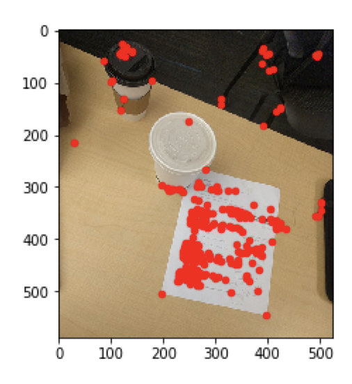
Here we compare the results of Lowe's on both the images. Noticed the reduced number of points (we went from 101 to 61 in this run) and that many have pretty good matches.
Part 4: RANSAC However, not all points-pairs are perfect. This is important because if any input points in generating the homography is incorrect, then the homography will be grossly incorrect and the image will not warp correctly. :(
To solve this, we use RANSAC! We take four point-pairs at random, generate the homography between them, and then test it out on all the input points from img1. If the resulting inverse warp leads you a set of points that is exactly like img2, then we've found our perfect homography! In practice, we ended up sampling randomly about 5,000 times for each image. To determine similarity, we just ran SSD from the output to img2 point's and selected the H that gave us the smallest value.
Have some images of final results! Which aren't much better than our original results, but at least we didn't need to click so dang much.
Tell us what you've learned! Dude, the concept of RANSAC is genius. I nearly screamed in class when we went over it. What a clever little algorithm!