San Fransisco from Lawrence Labs
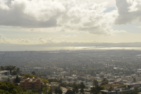
I took 3 sets of images for mosaic stitching and 2 pictures from online to practice image rectification.
San Fransisco from Lawrence Labs
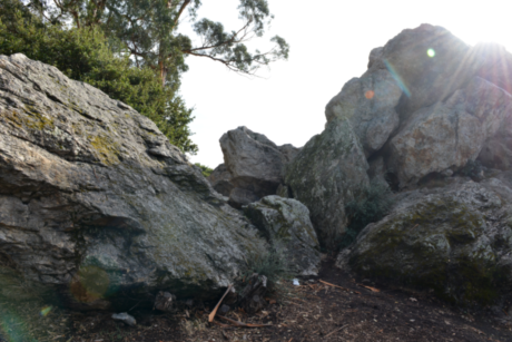
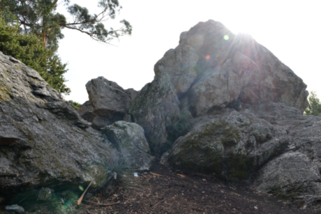
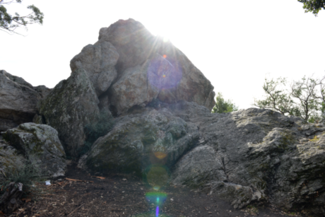
Indian Rock
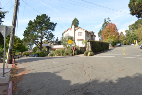
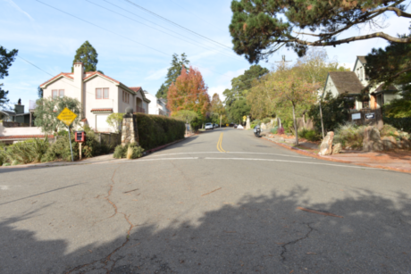
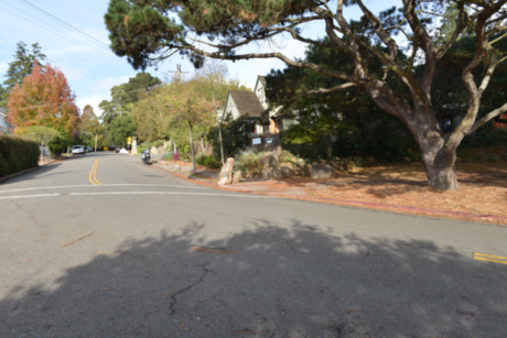
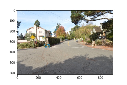
Northside Street
Balboa Park, Macbook
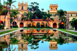

Homographies were recovered using ginput and manually selecting 10-16 points on each set of images to create correspondence. The warp matrix H was calculated as mentioned in class. In this section, I attempted to rectify two images to confirm that my homography recovery and image warping are correct. Below we see rectified frontal views of both Balboa Park and a Macbook.
Rectified Balboa Park, Rectified Macbook
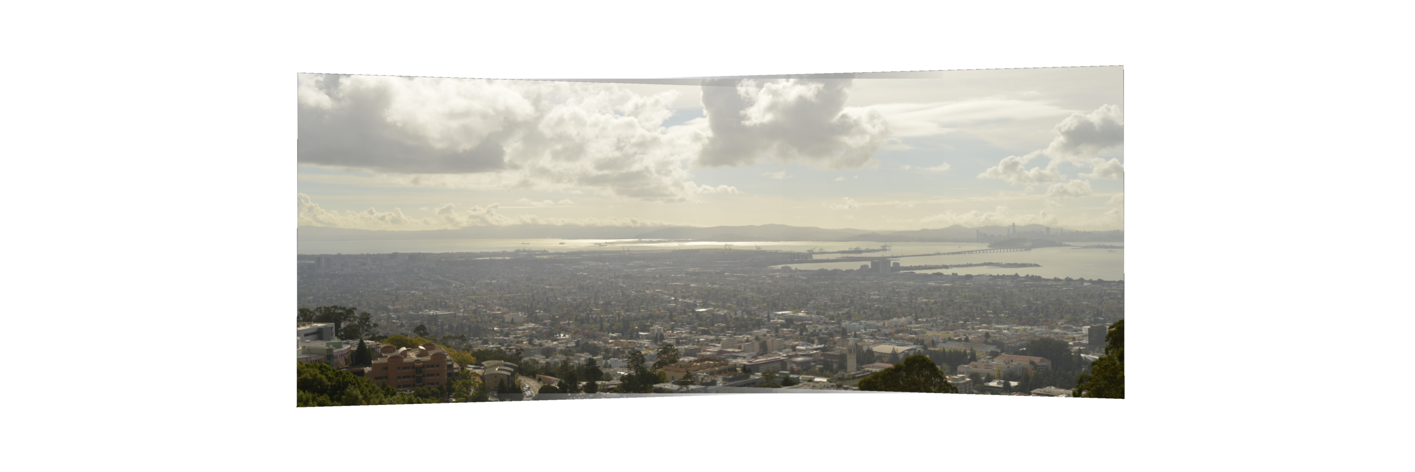
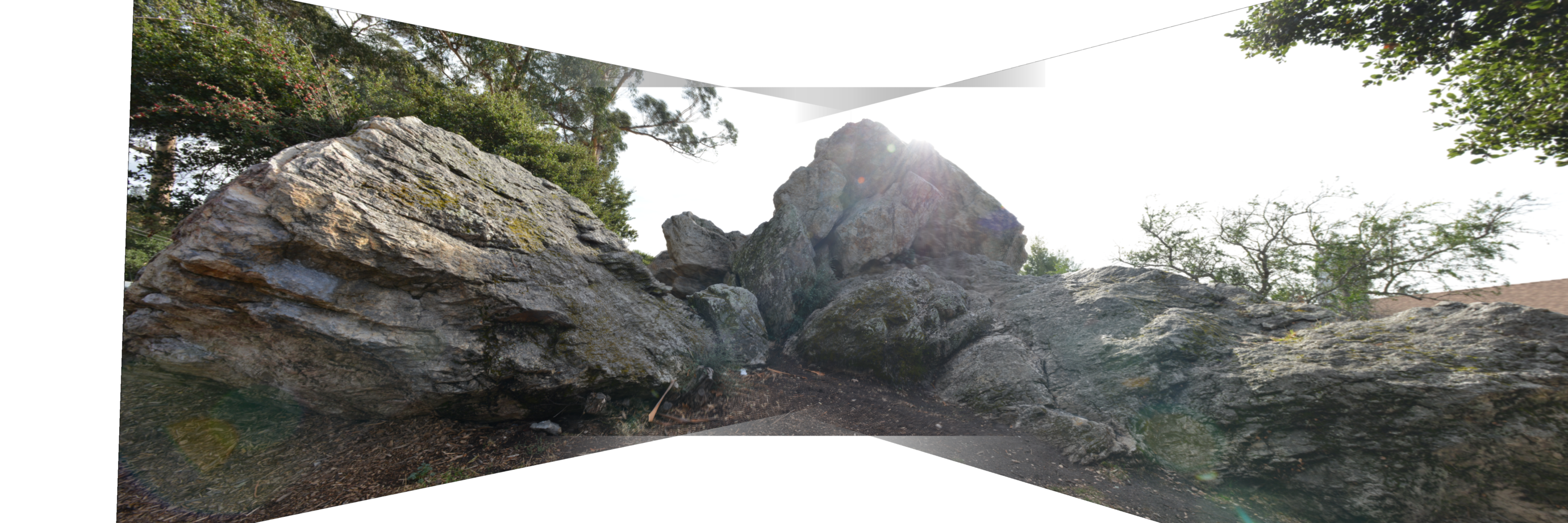
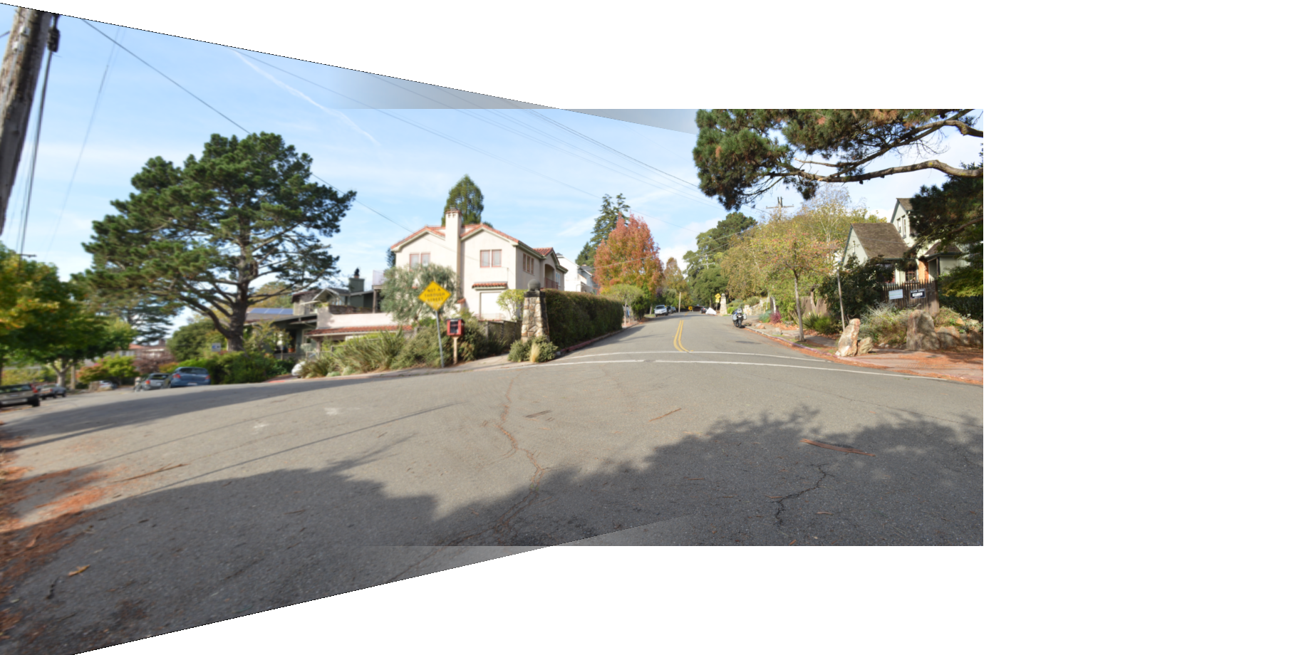
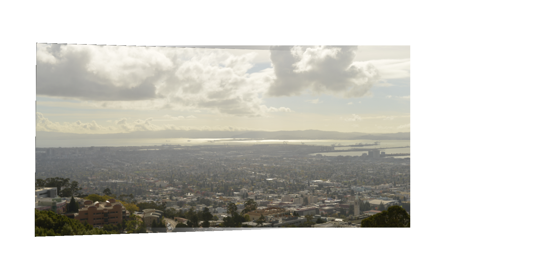
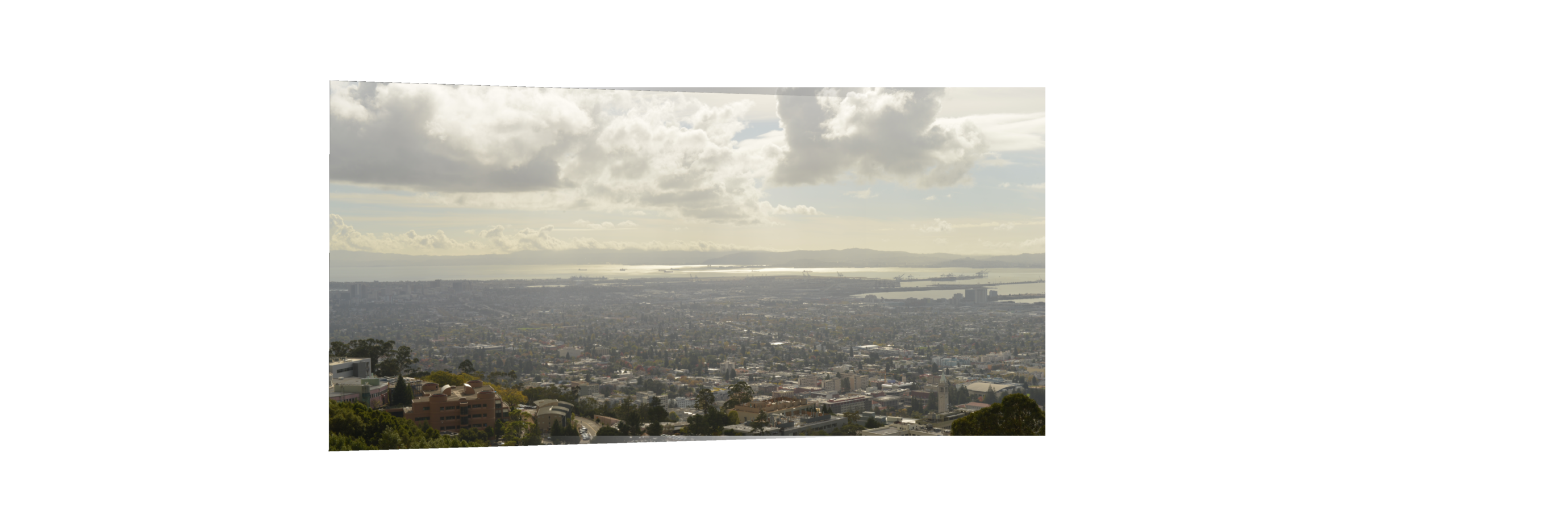
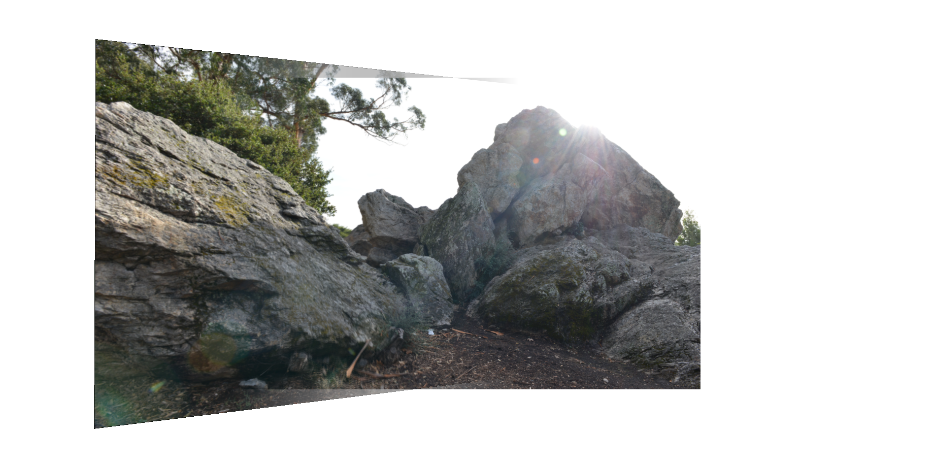
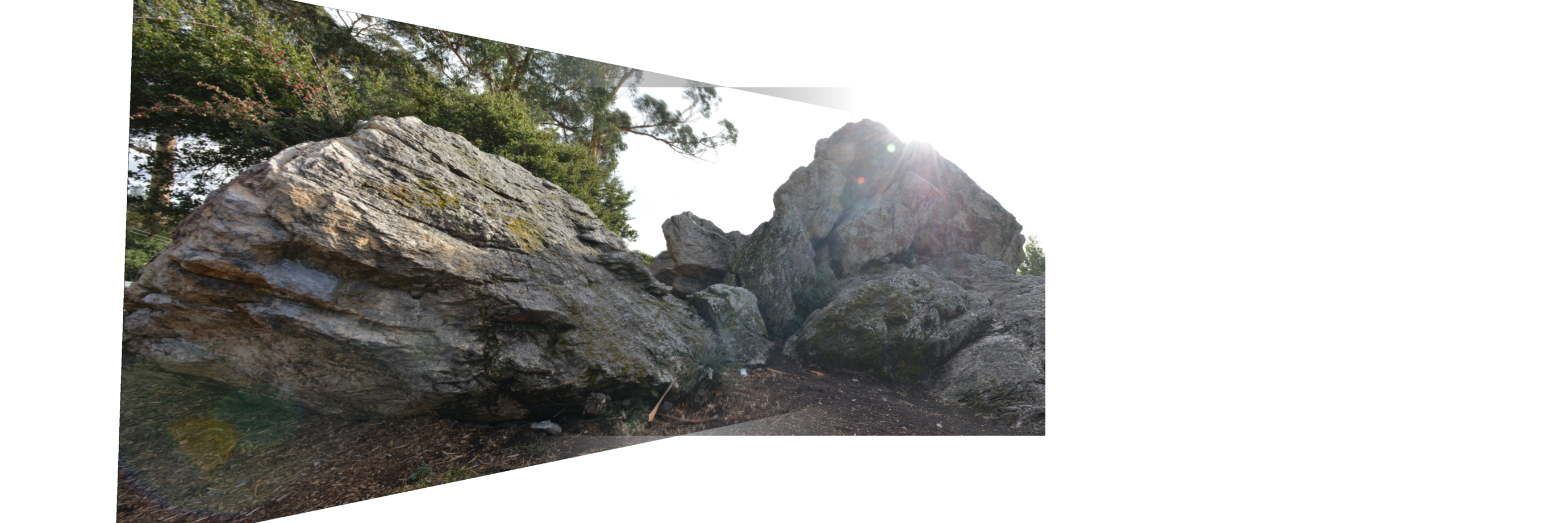
Since our homography recovery and image warping are correct, the last step is to combine our images into a mosaic. After correspondence is defined, this is done iteratively using by projecting each image onto the middle image as the base. Then, we use an alpha mask to linearly blend the overlapping areas to produce a smooth transition. The results for the rock and street mosaic are more extreme, as the focal length was a lot shorter. This contributed to greater warping and distortion across the mosaic. The mosaic of San Fransisco from Lawrence Labs turned out pretty nicely, as the focal distance was much longer.
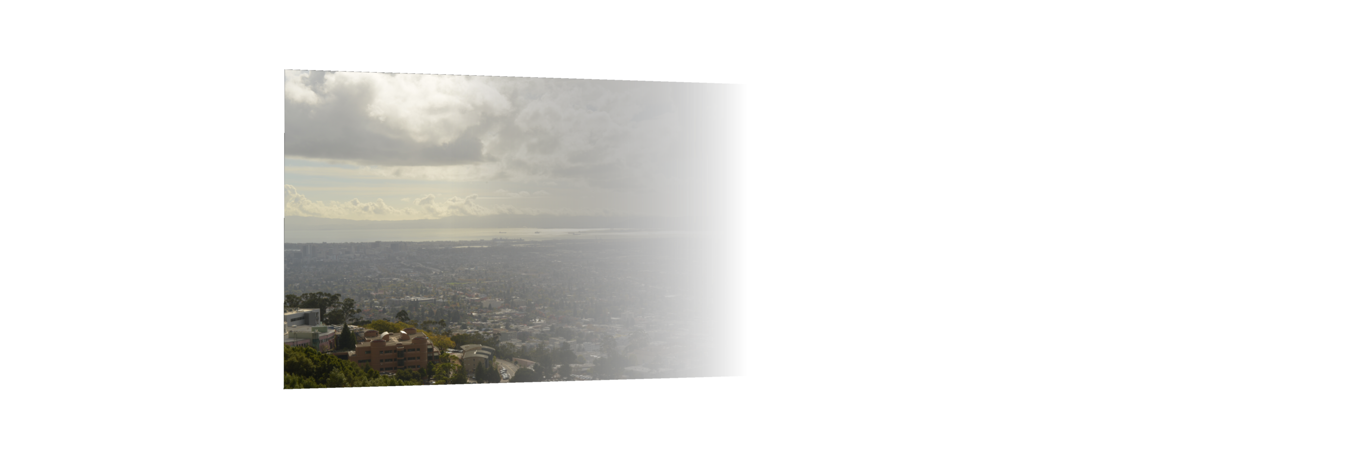
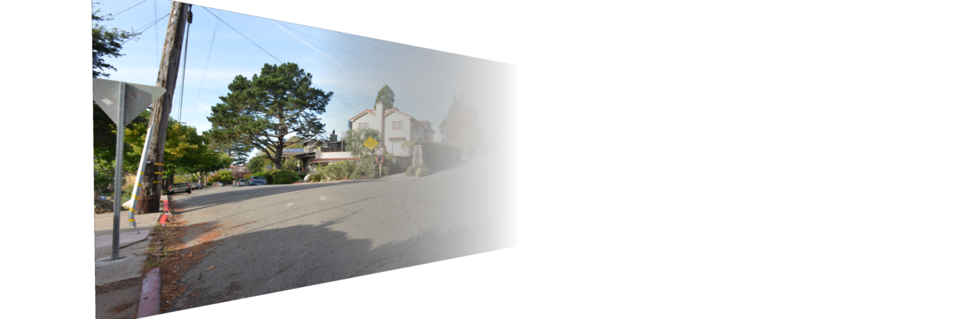
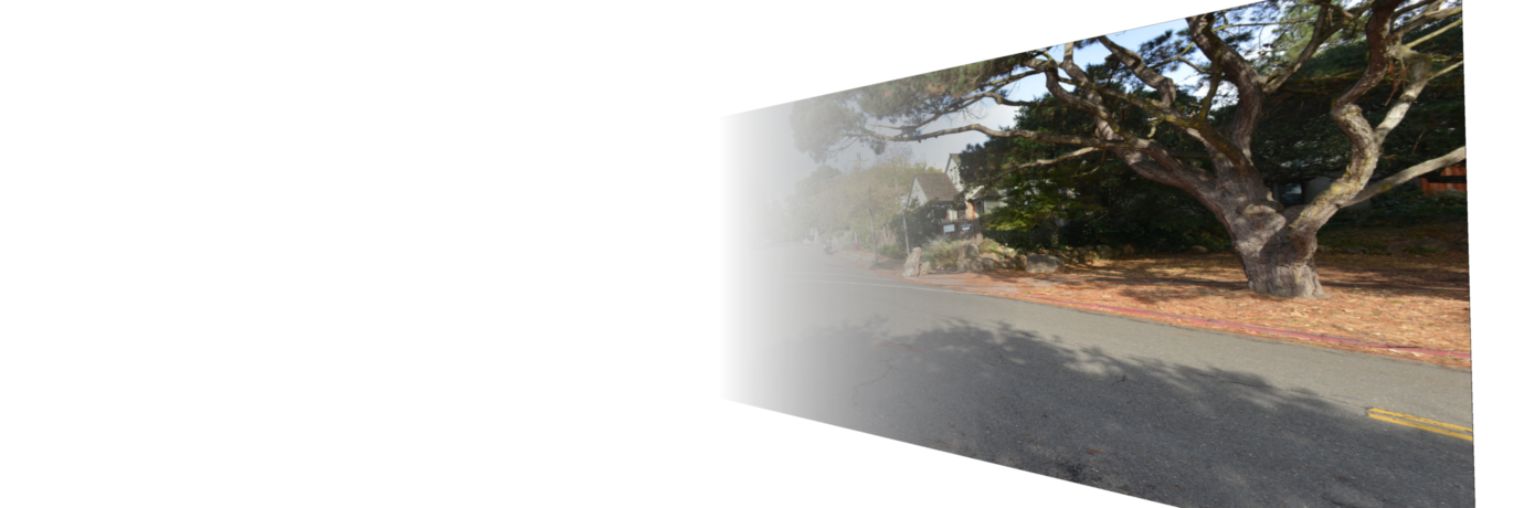
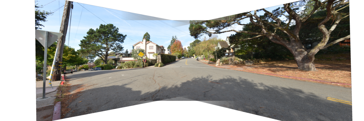
San Fransisco from Lawrence Labs
Left, right images warped onto the middle image with linear blending
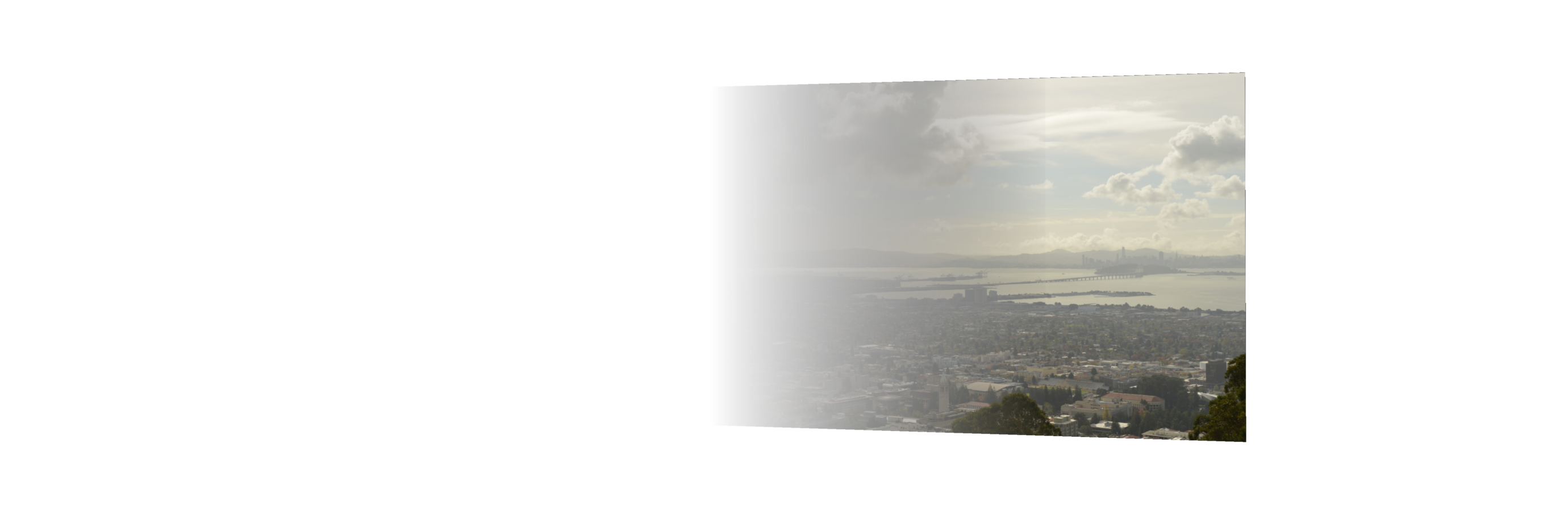
Resulting Mosaic
Indian Rock
Left, right images warped onto the middle image with linear blending
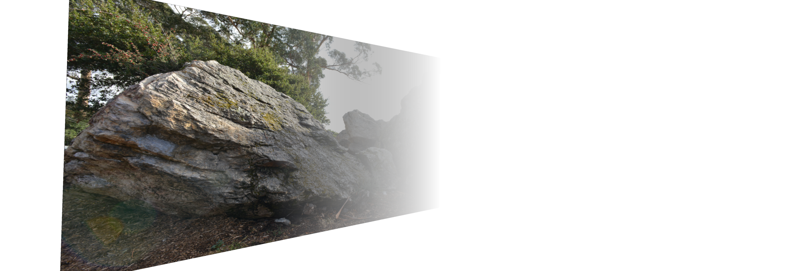
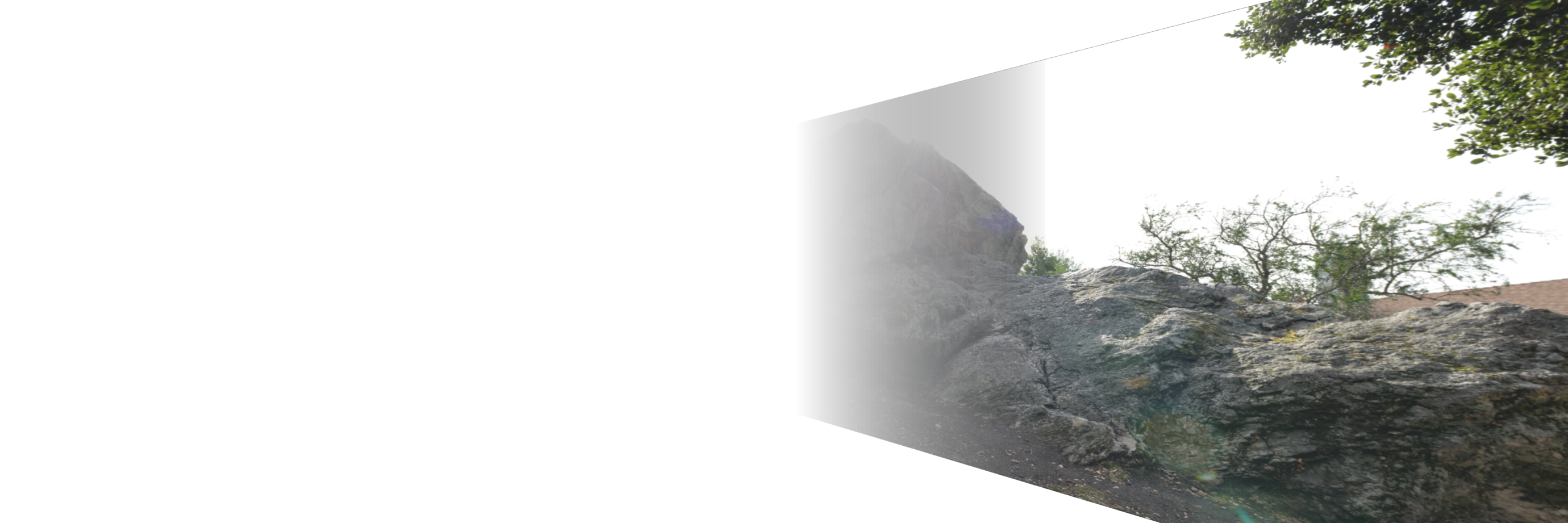
Resulting Mosaic
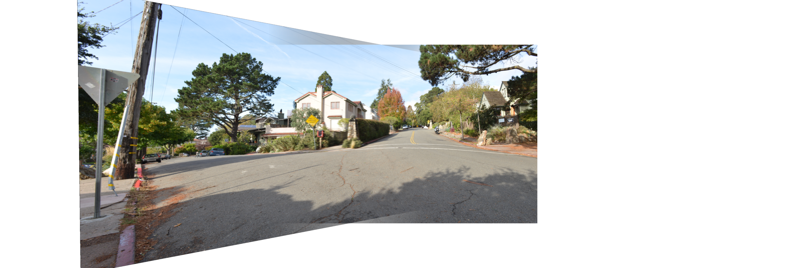
Northside Street
Left, right images warped onto the middle image with linear blending
Resulting Mosaic
A little math goes a long way! I didn't know the concept behind the panoramic software in our phones was that straightforward. This is a great application of linear algebra and demonstrates how useful it can be.
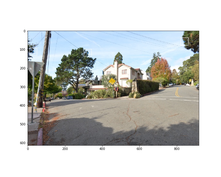
Manually defining correspondences is tedious. Let's automate this process by using harris points. A harris point, or corner, exists where the eigenvalues in the dx and dy directions are large. The code provided for detecting harris points noticeably returns many coordinates.
10000 Harris Points on Northside Street
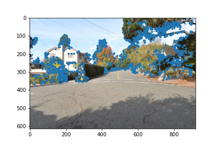
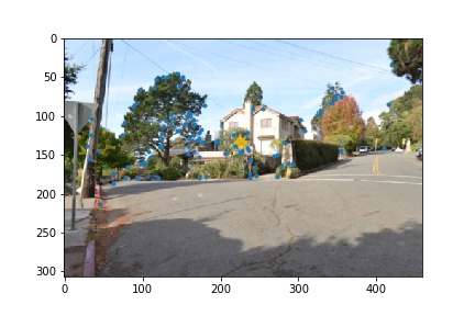
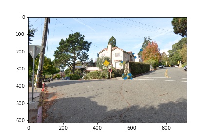
Evidently, there are a lot of harris points returned by the feature detection algorithm. The spacial proximity of these points relative to one another is pretty small. In other words, there are a lot of redundant features which will greatly slow down our algorithm later on. Instead of using all of these features, we will use only the most salient corners of the image determined by ANMS. For each point we find the largest radius in which it is the strongest point. Then we take the top x points, where x is a constant that we specify. The result is a significantly more spread feature set that reduces the feature space that we have to search for matches.
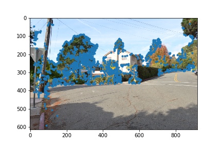
ANMS Harris Points on Northside Street
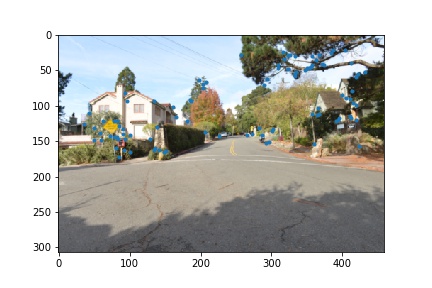
Now that our feature space is significantly reduced, we will construct a descriptor that summarizes the local characteristics of each feature coordinate. To do this, we implement MOPs. Around each feature coordinate, we take a 40x40 sample, then subsample this patch every 5 pixels to produce an 8x8 patch. Then we bias/gain normalize the patch values to have 0 mean and 1 standard deviation. Note that for simplicity, we ignore rotation invariance and the wavelet transform.
Example of 3 Multi-Scale Oriented Patches on Northside Street
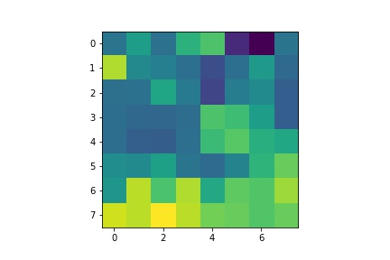
Corresponding Descriptors on Northside Street
Our feature descriptors are now arrays of length 64. To match the features, we follow Lowe's feature matching algorithm. For every feature vector on the first image, we compute the squared distance to all other feature vectors on the second image. Then we find the first nearest neighbor (1NN) and the second nearest neighbor (2NN). We use the ratio of 1NN/2NN to filter out inaccurate matches. The theory behind this metric is that if there is an accurate match, 1NN will be close to 0 and if there is no accurate match, both the first and second nearest neighbor will be about the same in terms of distance. Thus, if 1NN/2NN is close to 0 then we are likely to have an accurate match. If it is close to 1, then there is likely no accurate match. We choose a threshold value and only keep matches if 1NN/2NN is less than the threshold value. We do this for all pairwise features to obtain a set of matches.
The last step is to use RANSAC to remove the remaining outliers from our set of inliers. At each iteration of the algorithm, 4 corresponding features are sampled randomly without replacement. Then the homography matrix H is computed to map the first set of coordinates to the second set of coordinates. We take the distance between the mapped points and the expected points as a metric for if a pair is an inlier set or not. Out of all iterations, the largest set of inliers is taken and the homography matrix is recomputed.
Matching Features and RANSAC on Northside Street
Now we can simply apply the warp function using the calculated homography to produce our mosaic. We follow the same procedure of masking and linear blending as in part 1 in order to produce a stitched mosaic. Below are the resulting mosaics of both automatic feature matching and manual feature matching; the left image is automatically constructed and the right image is manually constructed.
Northside Street
San Fransisco from Lawrence Labs
Indian Rock
The automatic feature matching algorithm was a success! It produces nearly seamless mosaics that are on par with the mosaics that were created manually. The result is a much simpler method for stitching images together and a more automated process. One of the challenges of this project was finding the right threshold values for both ANMS, matching, and RANSAC. Each of these modules of the main algorithm require tuning for setting the correct threshold. If thresholds were too tight in one module, we potentially lost too many points in the final step. This would result in an inaccurately blended image. But when thresholds are tuned properly, automatic mosaic stitching is very robust. Even though portions of the algorithm are not deterministic, the algorithm is able to consistently find good correspondences between the images and correctly stitch them into a mosaic. Ultimately, this project incorporated almost all of the concepts covered throughout the class. It was a great way to apply everything we had learned into a project that summarizes the course content.