This is the first part of a project involving stitching together photographs to create larger composite images. In this part, we capture source photographs, define correspondences between them, warp them to the same shape, and composite them.
For creating image mosaics, we first capture multiple images: either by shooting them from the same point, or by capturing a planar surface from different poitns of view. We then want to be able to transform one image into another, or both into a common perspective. This transformation is a homography defined by the relationship
This can be rearranged into the equations
Which are reformulated as a linear system.
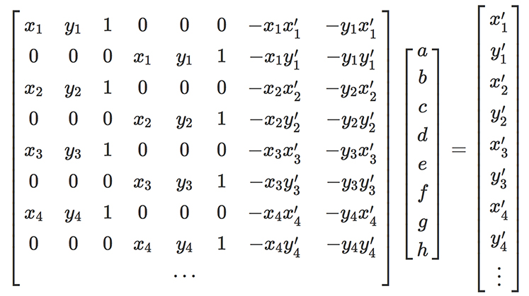
Each x/y pair represents a point in the first image, and the corresponding x'/y' pair is the same point in the second image. This system is precisely determined given 4 pairs of points. However, to make the matching more robust, I used more points and solved the system using least squares.
The first test of my algorithm was image rectification, which warps images in order to make specified surface planes to be frontal-parallel. Since there is only one image in this situation, the corresponding points were manually defined to be rectangular. In this manner, the original image was warped into the specified rectangular shape.
For image mosaicing, I took photos from one point at different angles. I chose common points between the two images, defined one image to be the reference, and warped the second image to match the first one. The first result for each mosaic shows the results of naively stacking the two images together. This doesn't work too well because it doesn't account for changes in exposure, color balance, and other variations that can occur between the two photos. The second result shows the results of linear blending, which applies a weighted average to overlapping pixels depending on their coordinates. This makes the overlapping regions transition more smoothly between differing colors in the two source images.
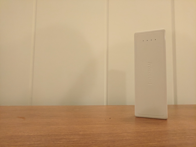 Power bank left angle
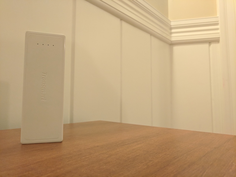 Power bank right angle
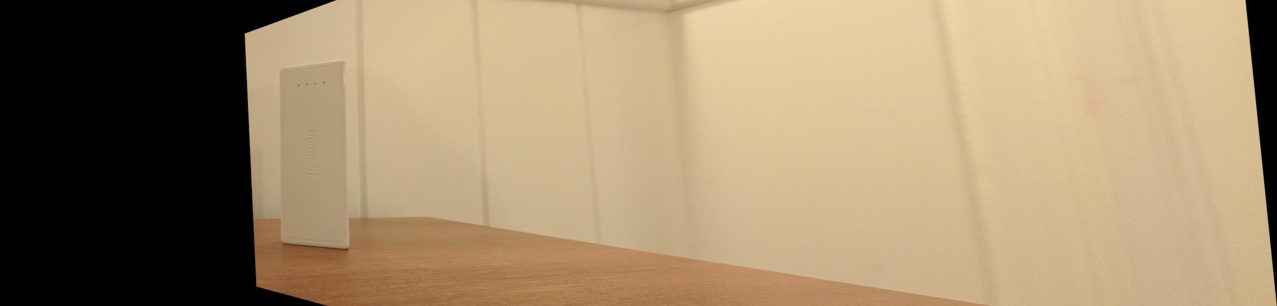 Power bank right angle transformed
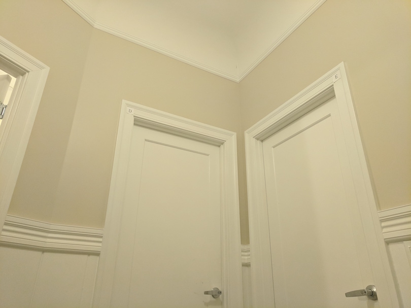 Doors left angle
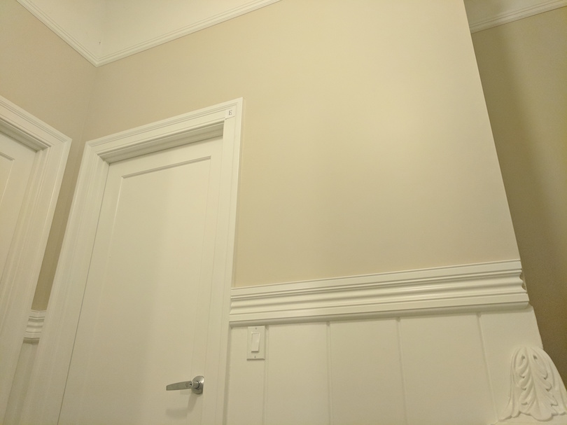 Doors right angle
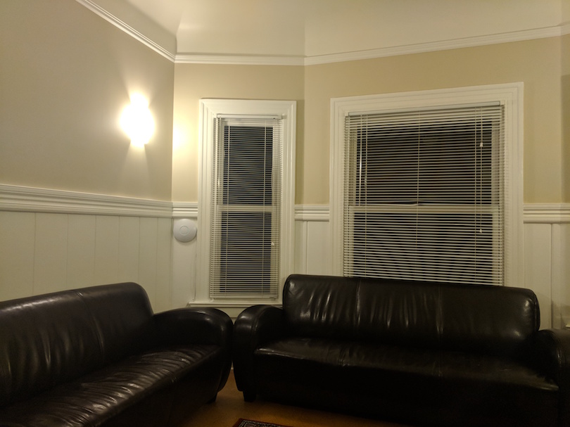 Living room left angle
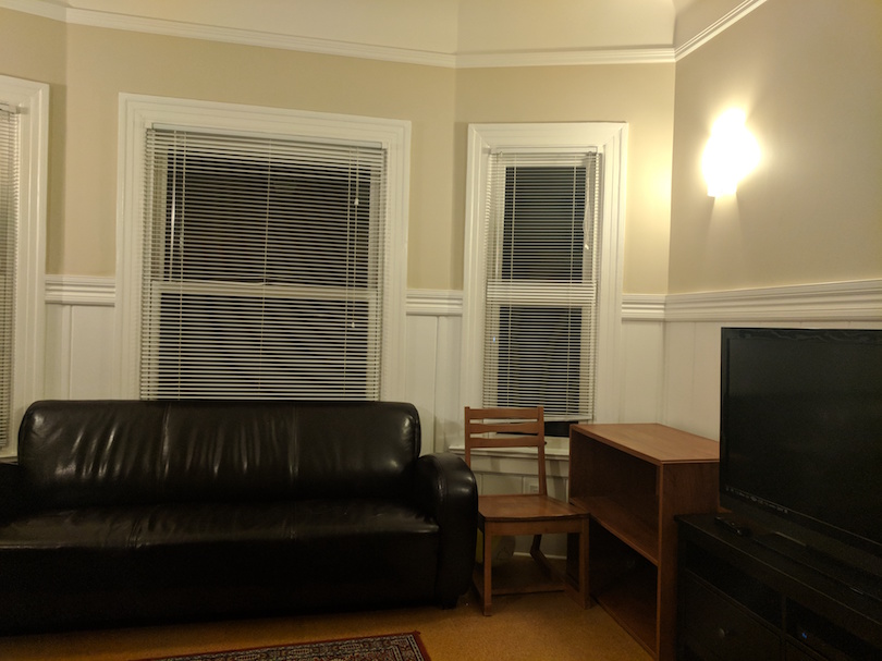 Living rooms right angle
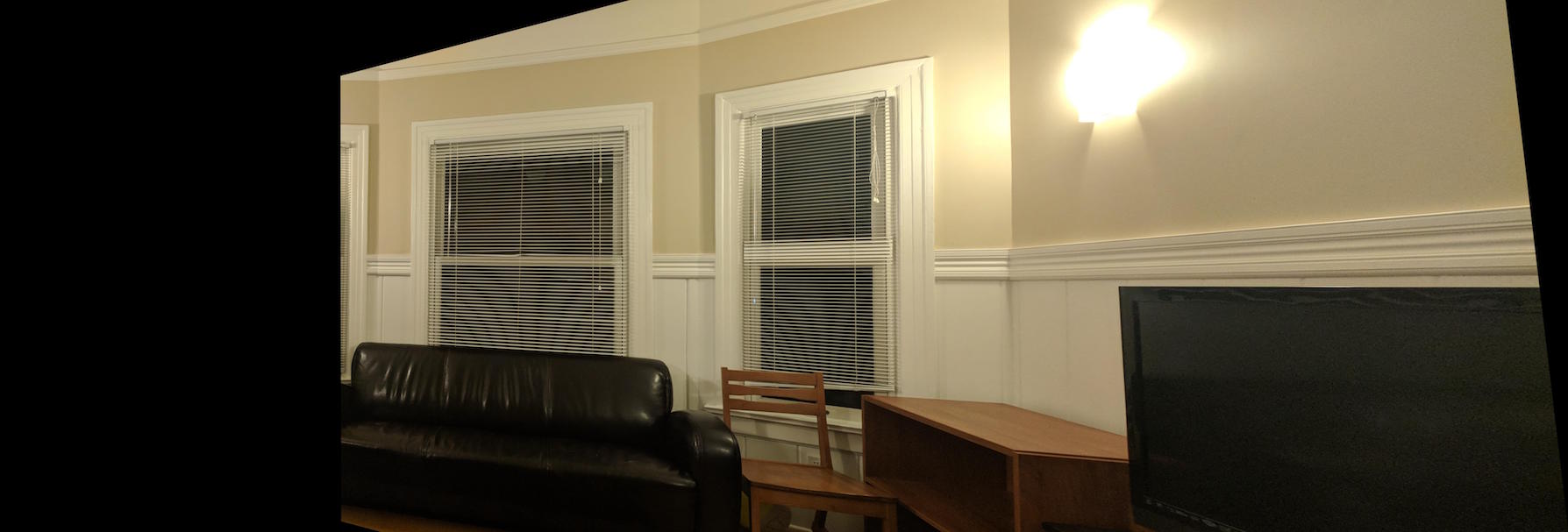 Living room right angle transformed
From this project, I learned that making panoramas with multiple images is definitely possible, but it involves keeping track of many minute details about linear algebra and image blending. I also learned that I really enjoy computational photography, and I'm looking forward to the next part of this project!
In Part 2 of this project, we automate the correspondence-finding portion from Part 1 of the project. This allows us to create panoramas automatically.
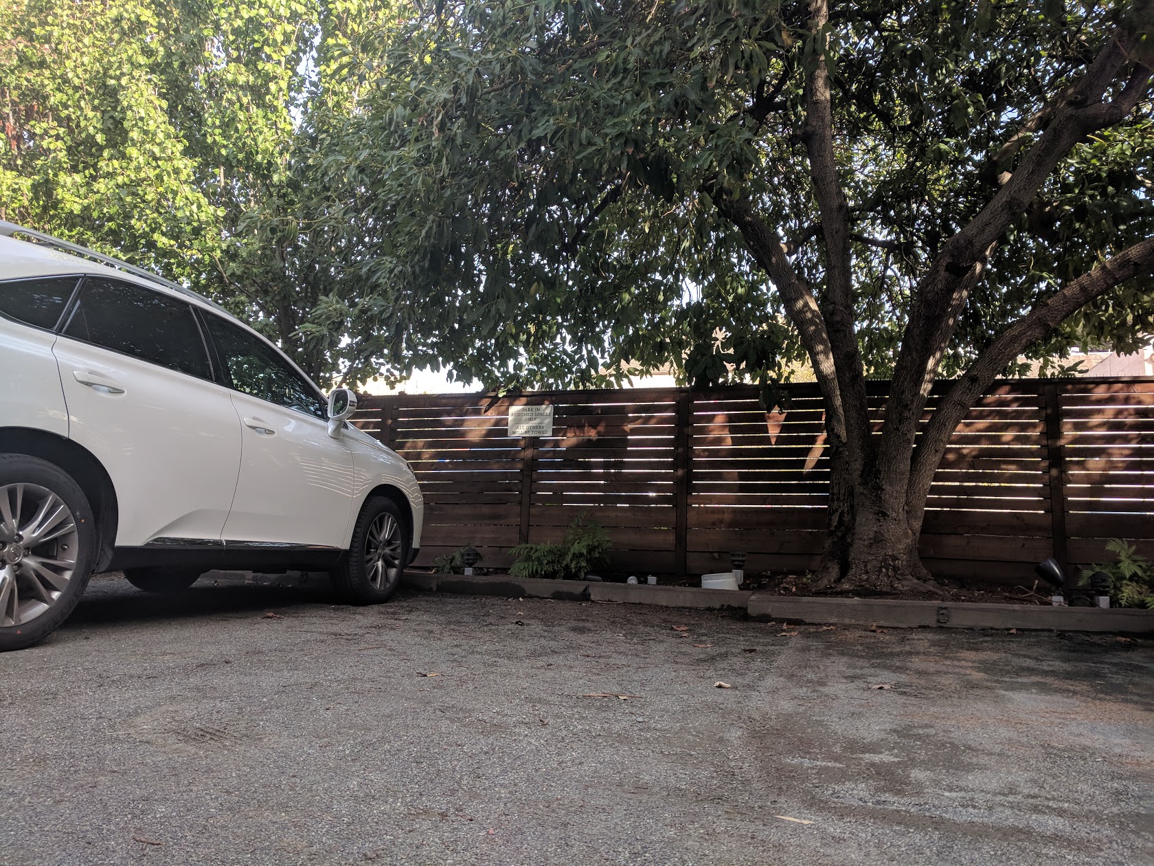 Parking lot left angle
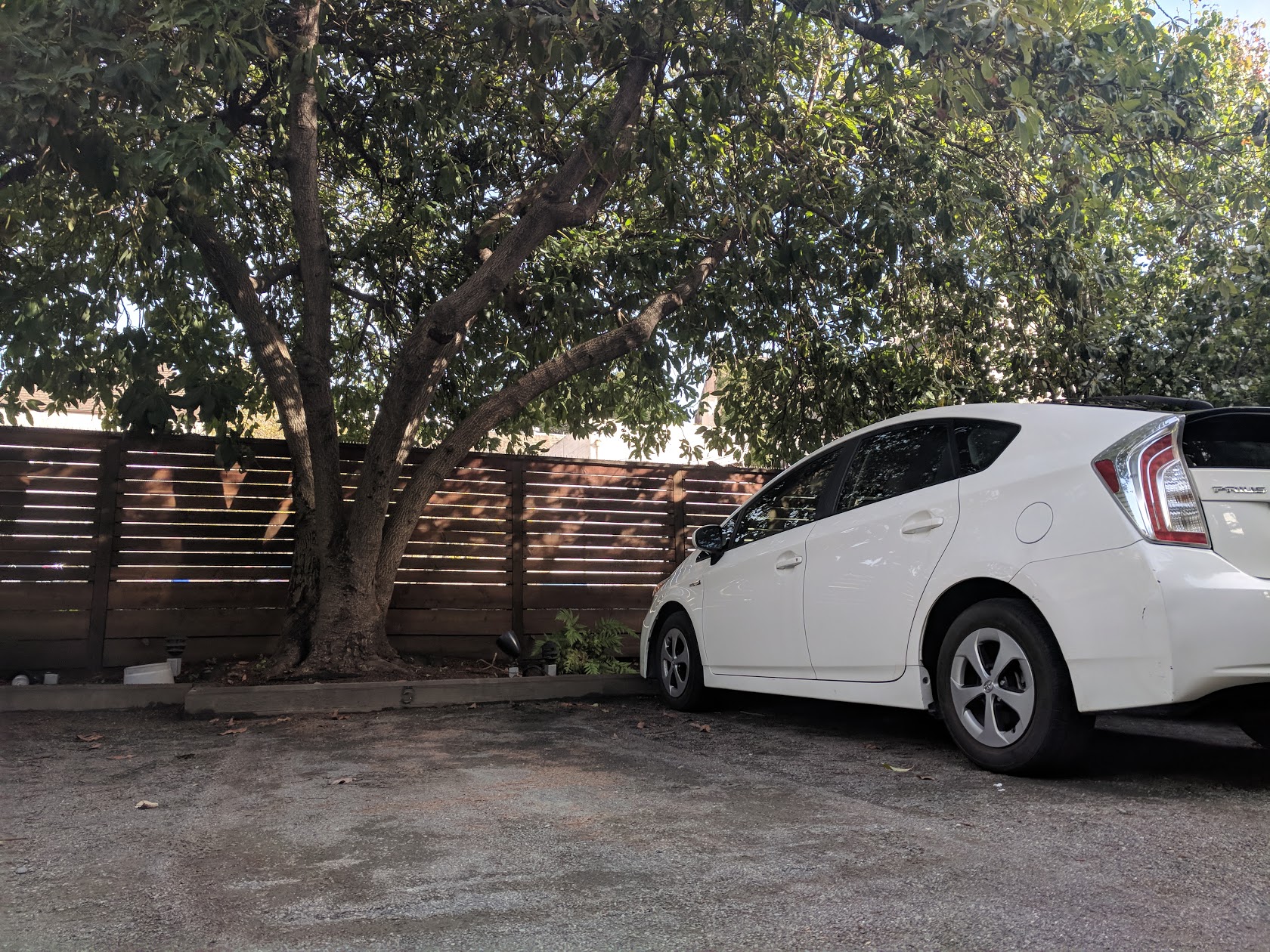 Parking lot right angle
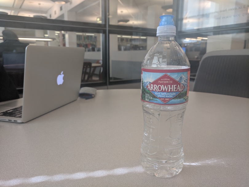 Water bottle left angle
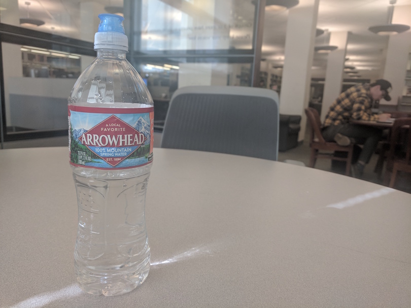 Water bottle right angle
Doors left angleDoors right angle
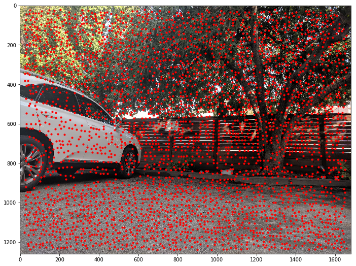
First, we want to automatically detect corner features in our images. The interest points we use are Harris corners, which are found using a grayscale version of our input image
 Parking lot left angle
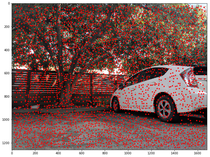 Parking lot right angle
 Water bottle left angle
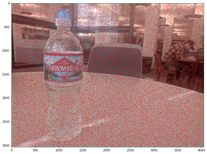 Water bottle right angle
 Doors left angle
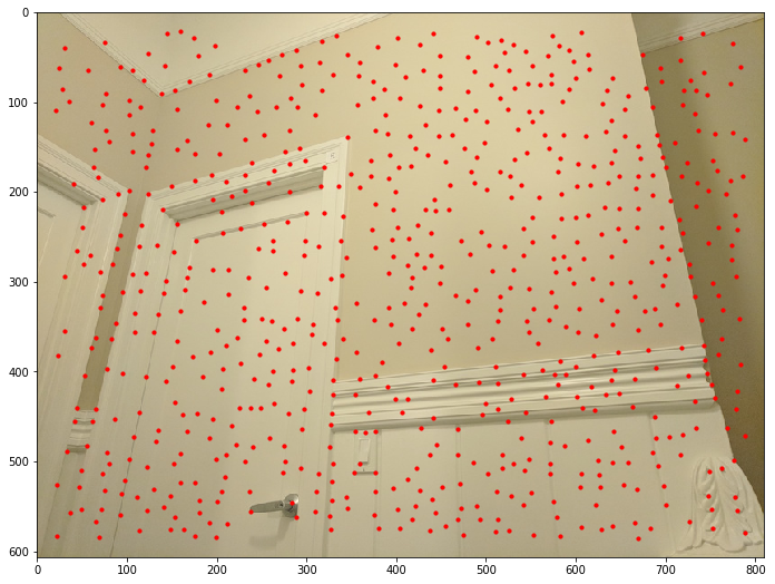 Doors right angle
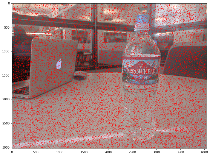
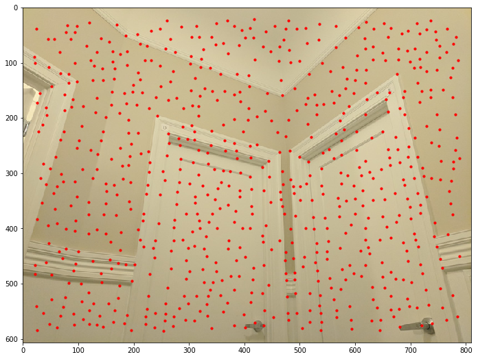
We get between several hundred to around 20,000 interest points from the previous part. We want to restrict the number of points we consider so that we only use meaningful ones and reduce computational cost, but we must also ensure that the selected points are well-distributed over the image. In order to do this, we use an adaptive non-maximal suppression strategy that suppresses points close together.
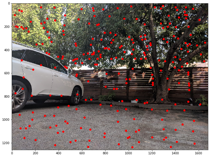 Parking lot left angle
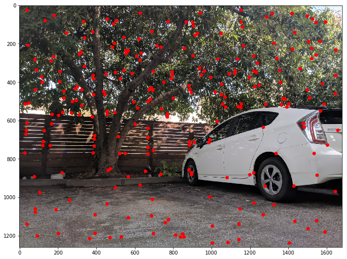 Parking lot right angle
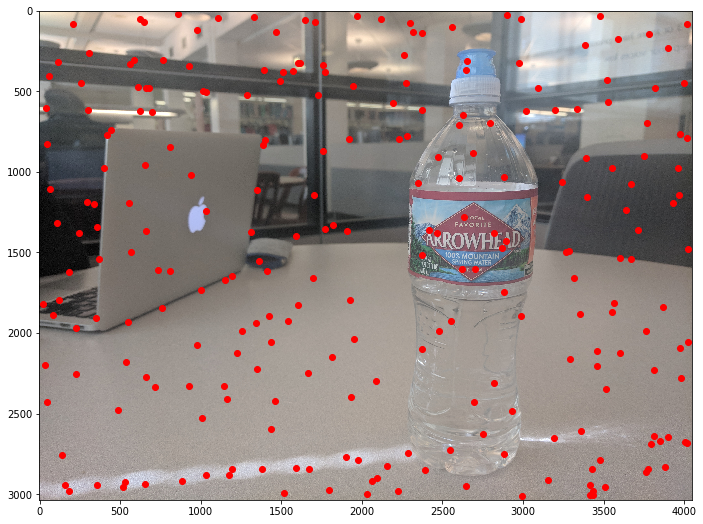 Water bottle left angle
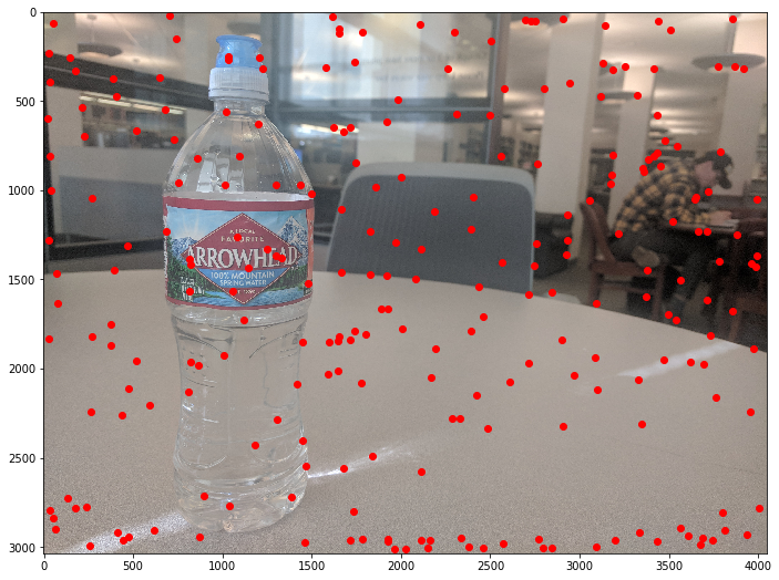 Water bottle right angle
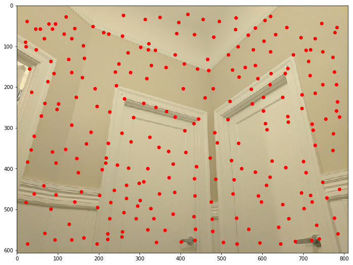 Doors left angle
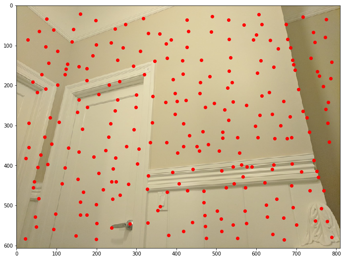 Doors right angle
We extract axis-aligned 8x8 patches for each of the ANMS points that we have. These patches are sampled from larger 40x40 windows, which gives us a large blurred descriptor around each interest point. We reshape these patches into length-64 vectors that are then bias/gain normalized.
We have now computed feature descriptors for a pair of images. For each descriptor in the first image, we find its nearest and second-nearest neighbor in the other image. Our metric for nearness is the sum of squared distances between corresponding feature descriptors. Then, if the ratio of 1-NN SSD to 2-NN SSD is below a certain threshold (I generally used 0.4), then we consider our original point and its nearest neighbor to be a match.
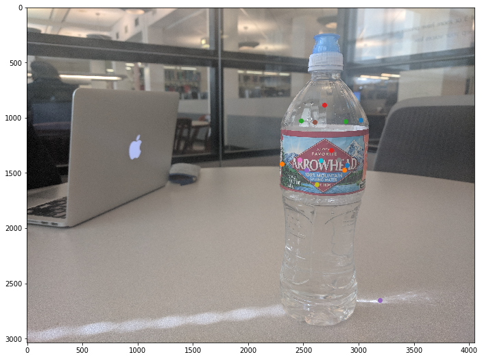
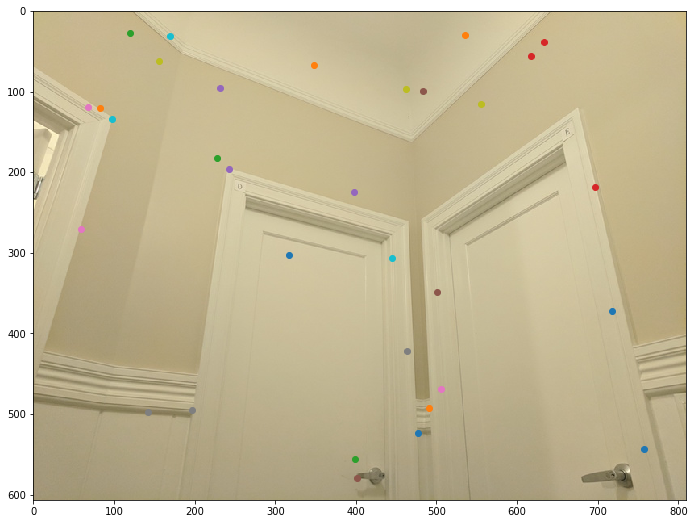
In the following images, points with matching colors between image pairs are considered to be matches by our algorithm. You can see that there are often many matches, but there are always some mismatched points.
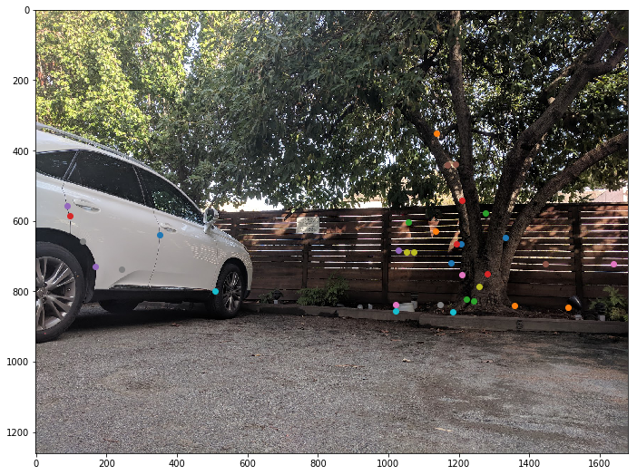 Parking lot left angle
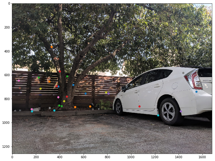 Parking lot right angle
 Water bottle left angle
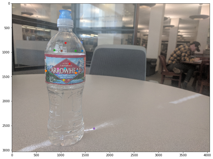 Water bottle right angle
 Doors left angle
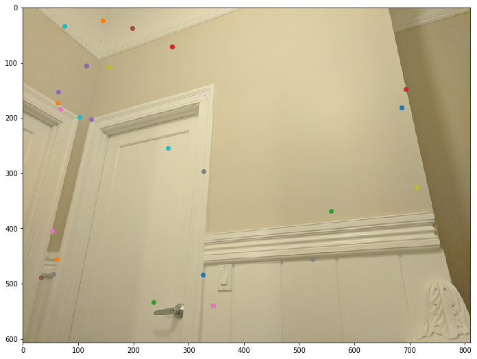 Doors right angle
We now want to compute a homography to transform one image into the other. For this, we use RANSAC. The basic process first involves randomly choosing four matching pairs of points. Compute a homography using these 4 points. This homography gives us predicted transformed locations for the first point in each pair. Then, for each of the corresponding second points, compare its location to that given by the homography. We compute the number of points that fall within a certain threshold of the actual positions and call these inliers. We run this process 10,000 times and choose the sampled homography that returns the most inliers. Once we have this best homography, we tune it using all of its inliers to get a final homography matrix.
We compare the results of our automated stitching procedure to those done with manual point picking (as in part A of this project).
For the parking lot, both automatic and manual stitching produced very good results with almost unnoticeable artifacts. The two results are almost identical.
For the water bottle, automatic stitching did a pretty good job, but manual point selection does slightly better. We can see especially to the right of the bottle cap where there are aberrations in the automatic image that are not present in the manual image. One factor in this is that when feature matching is done for the bottle images, almost all of the points fall on the label of the bottle. This makes the automatic stitching work very well for the region of the image that contains the bottle, but surrounding parts of the image don't get matched as well.
For the doors, automatic stitching clearly does not work as well as manual stitching does. One reason for that is that there are many repeating features in the images, such as corners of the door and long edges. This causes many of the "paired" features to not actually match up, which causes automatic stitching to work less well.
For the charger, automatic and manual stitching produce basically identical results.
I found this project really awesome. It was great learning what makes automatic stitching work. The coolest thing I learned is how correspondences between images can be automatically found even when the photos contain many different pieces and are taken at different angles.
 Original
 Rectified
 Original
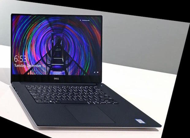 Screen rectified
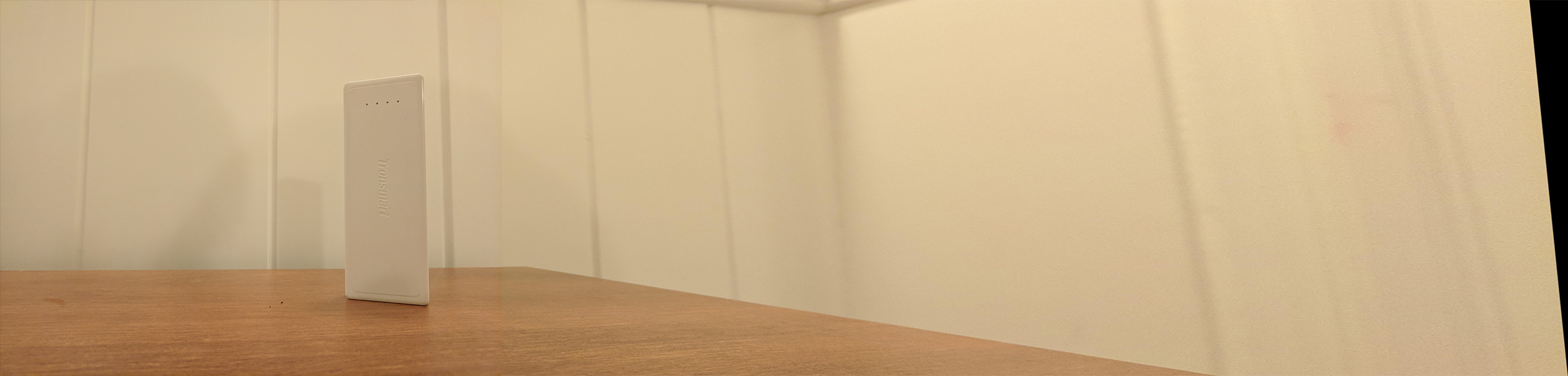 Mosaic naively stacked
 Mosaic linearly blended
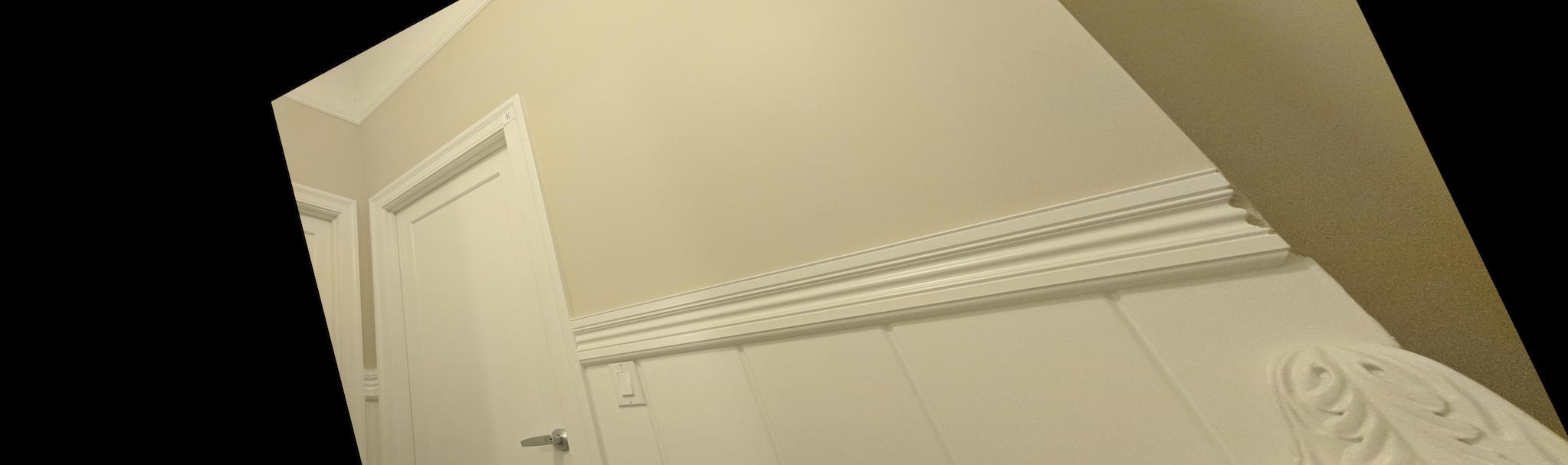 Doors right angle transformed
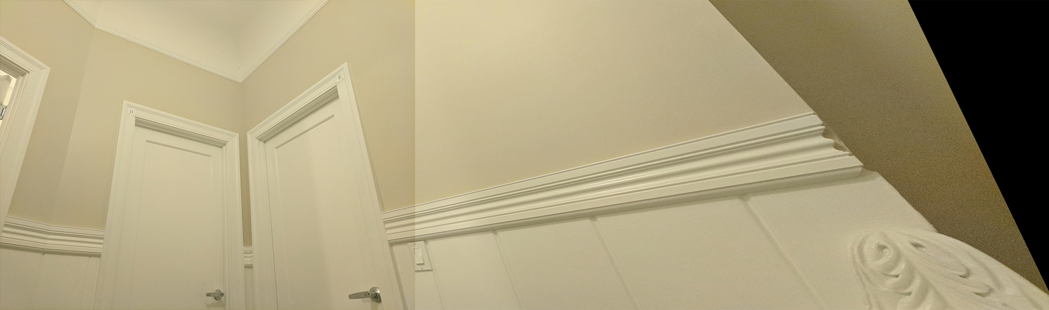 Mosaic naively stacked
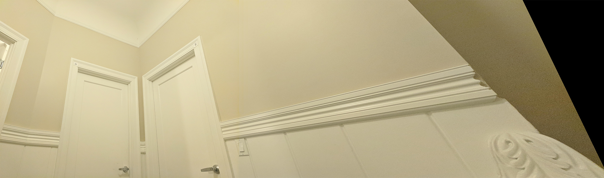 Mosaic linearly blended
 Mosaic naively stacked
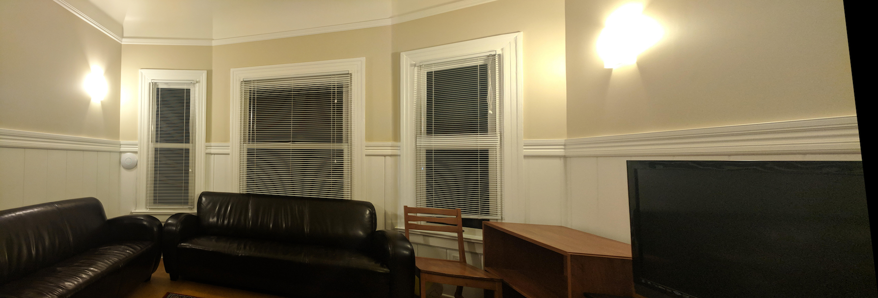 Mosaic linearly blended
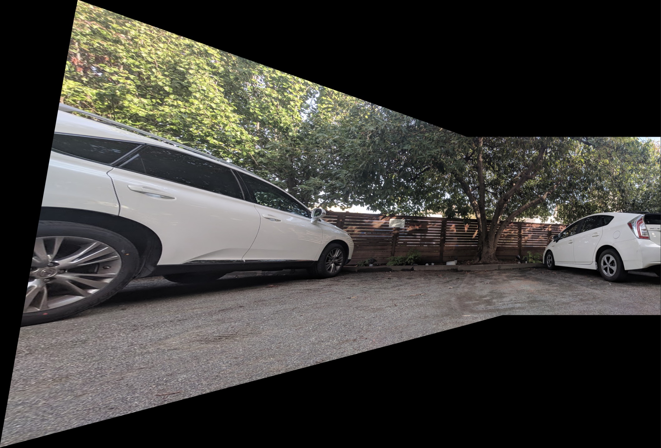 Parking lot automatic
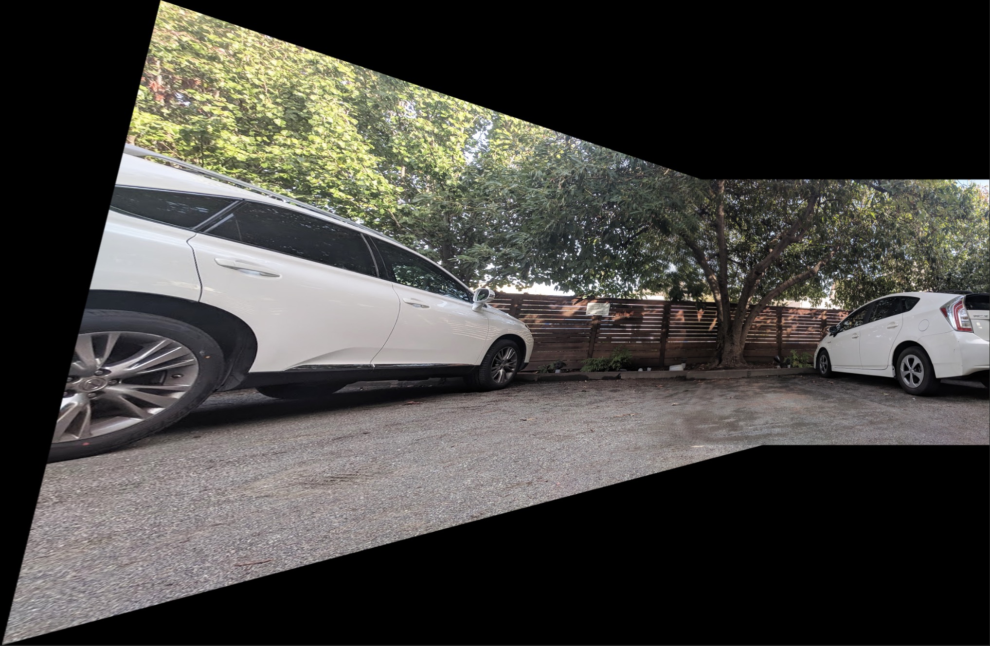 Parking lot manual
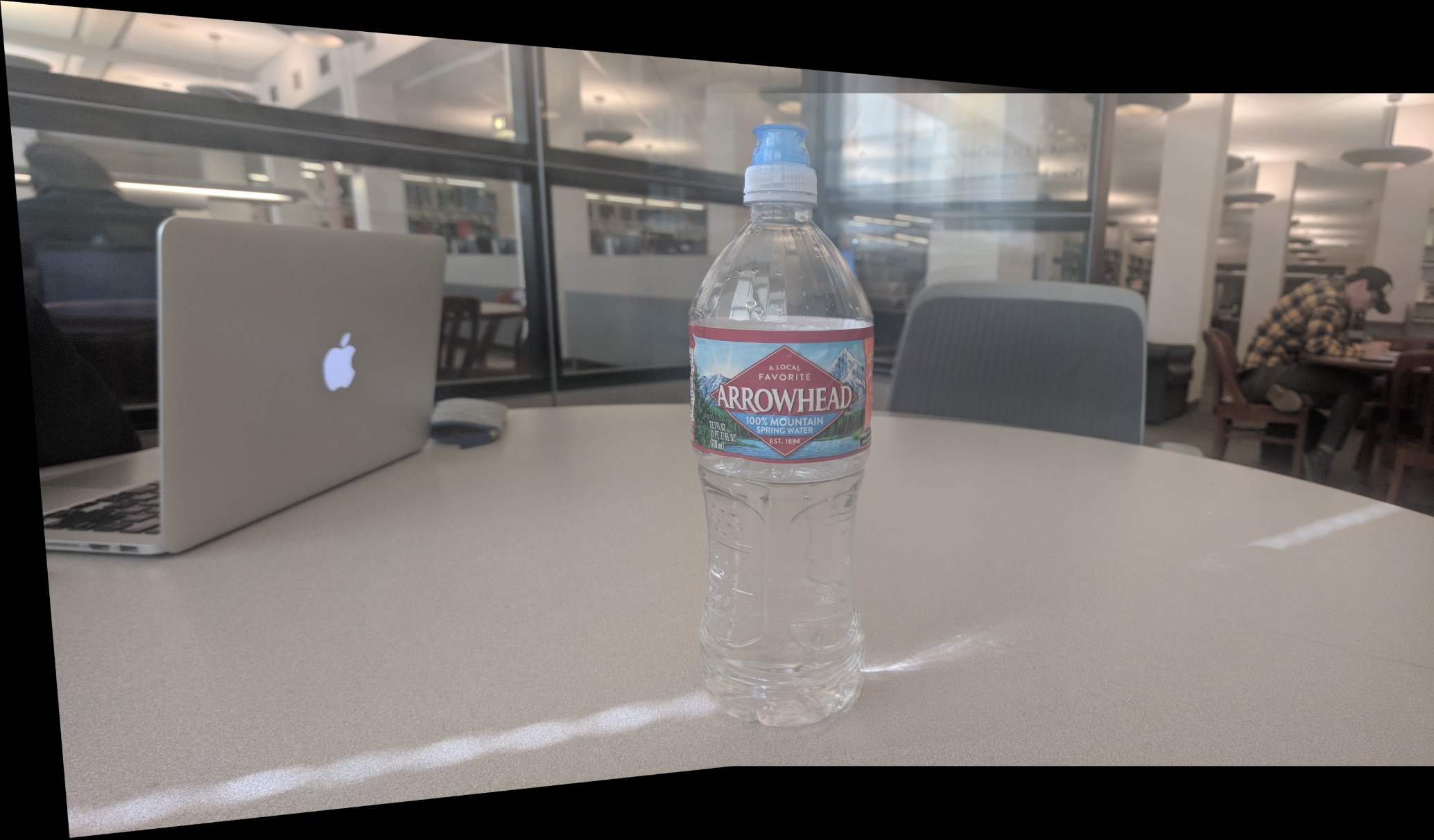 Bottle automatic
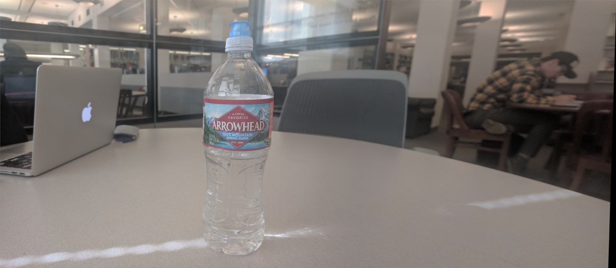 Bottle manual
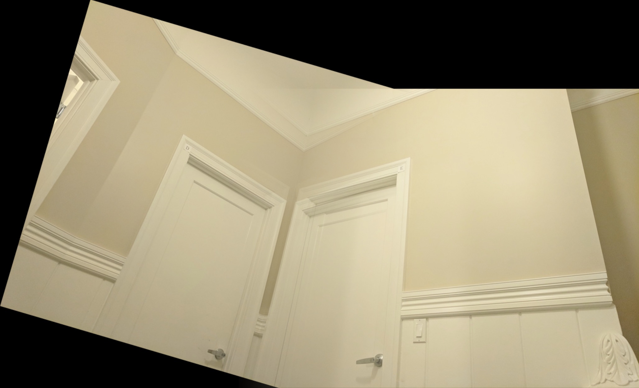 Doors automatic
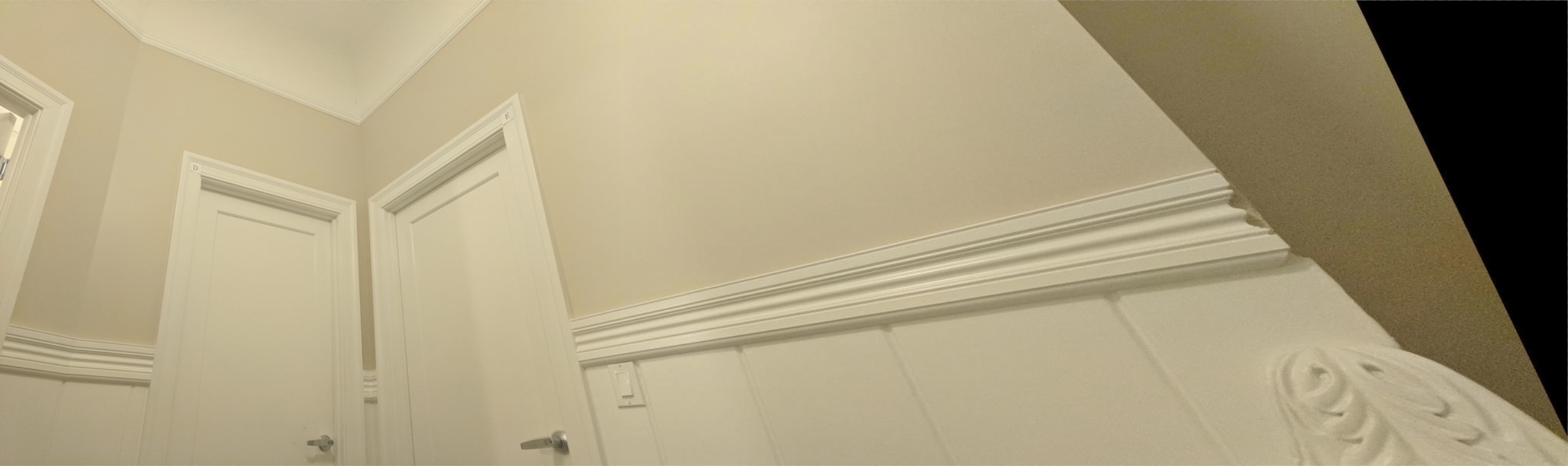 Doors manual
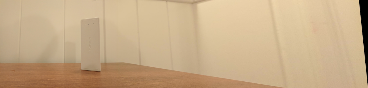 Charger automatic