Introduction
This project has two main parts. The goal of the first part is to explore different aspects of image warping with a cool application - image mosaicking. I will take two or more photographs and create an image mosaic by registering, projective warping, re-sampling, and compositing them. Along the way, I will demonstrate how to compute homographies based on manually selected correspondences, and how to use them to warp images. The goal of the second part is to find robust correspondences automatically.
Homography Theory
 |
|---|
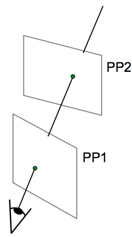
Projection – mapping between any two PPs with the same centre of projection |
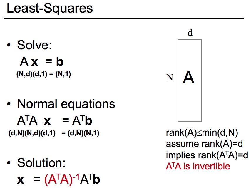
To recover the homographies between 2 images, we need at least 4 correspondences. This is because homographies can be expressed by the following transformation with 8 unknowns.
 |
|---|
Homography transformation |
Notice the above equation is not in b = Ax form. For the sake of easier computation, we rearrange the matrix as the following b = Ax form:
 |
|---|
Homography transformation |
However, one complication is that the 4 points selected might be noisy. So we should select more than 4 points and minimise the matrix rather than solving it directly.
 |
|---|
Solution to minimisation1 |
1 Image Rectification
1.1 Theory
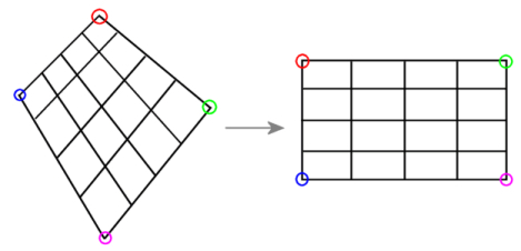
From the homography transformation theory about, to rectify an image, I take a single image of a planar surface. Then I apply the warping to transform 4 points into to a frontal-parallel plane.
 |
|---|
Idea behind rectification
1.2 Results
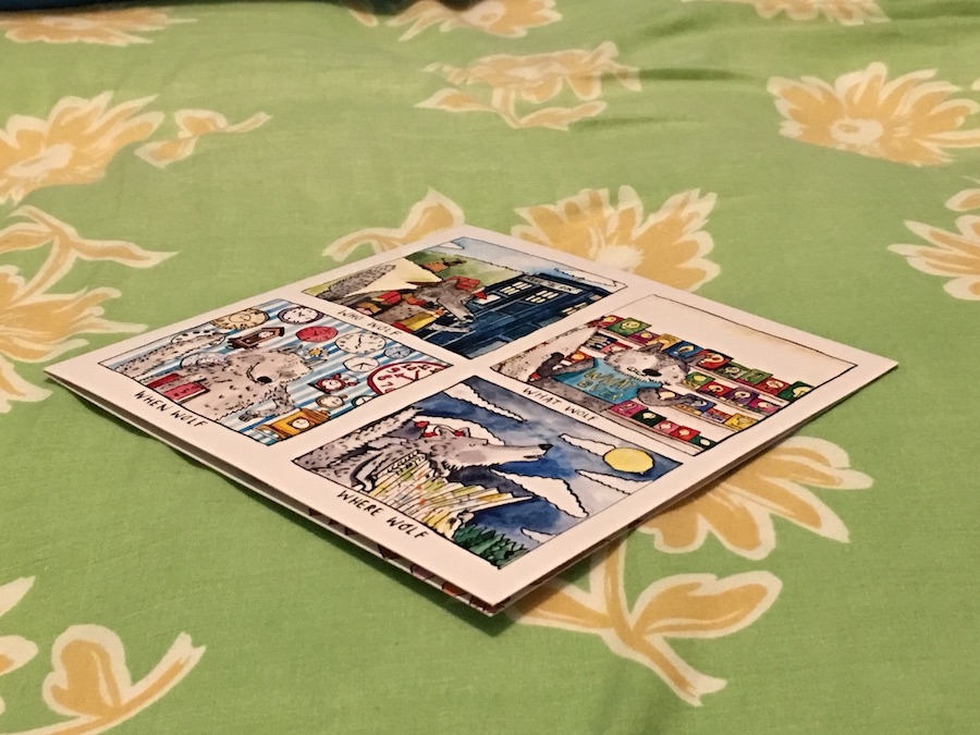
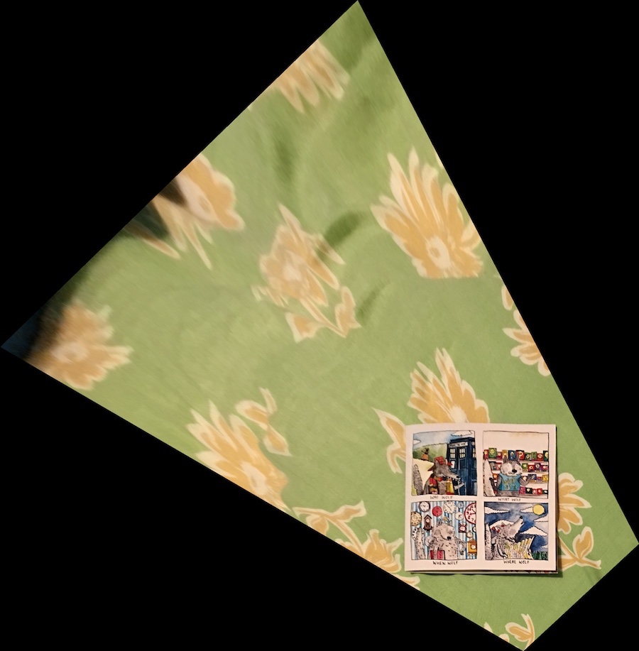
As the following images, I rectified the original into a top-view.
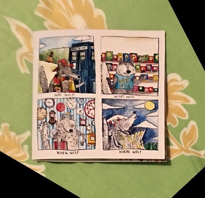
Whovian
 |
 |
|---|---|
| Original | Rectified |
 |
|---|
Cropped Result |
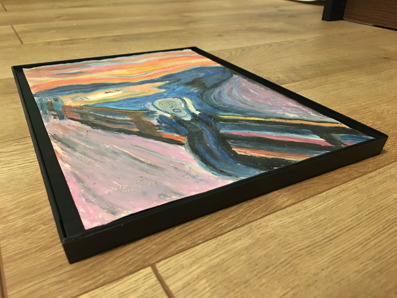
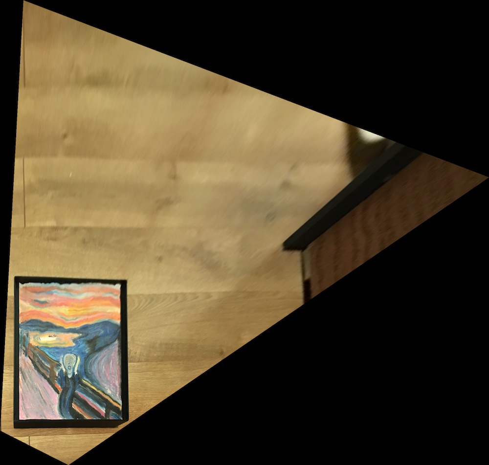
Scream
 |
 |
|---|---|
| Original | Rectified |
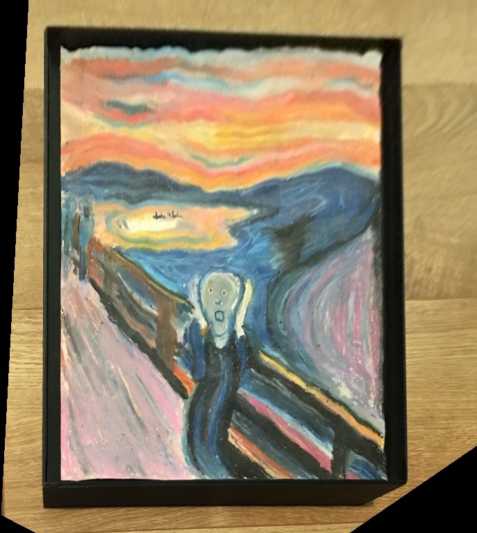 |
|---|
Cropped Result |
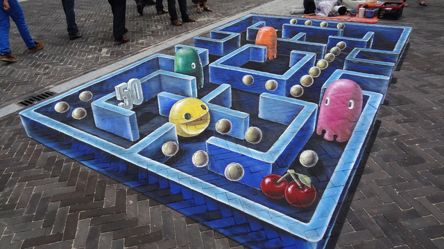
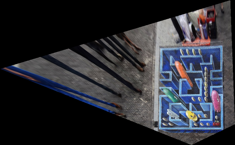
Pacman
 |
 |
|---|---|
| Original | Rectified |
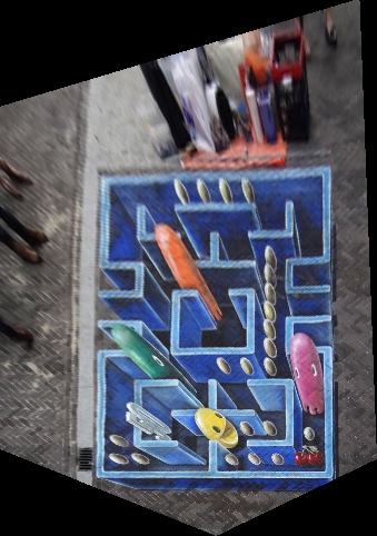 |
|---|
Cropped Result |
2 Blending Images into a Mosaic
2.1 Theory
Warp the images so they're registered and create an image mosaic. I left one image unwrapped and warp the other image into its projection. Then I blended the images together.
I first picked correspondences from both images.
 |
|---|
Correspondences
Then I computed homographies and warped the first image into the other projection.
 |
|---|
Warped image
After that, I padded both images to prepare for blending.
 |
 |
|---|
Padded images
Finally I blended the two images
 |
|---|
Padded images
2.2 Results
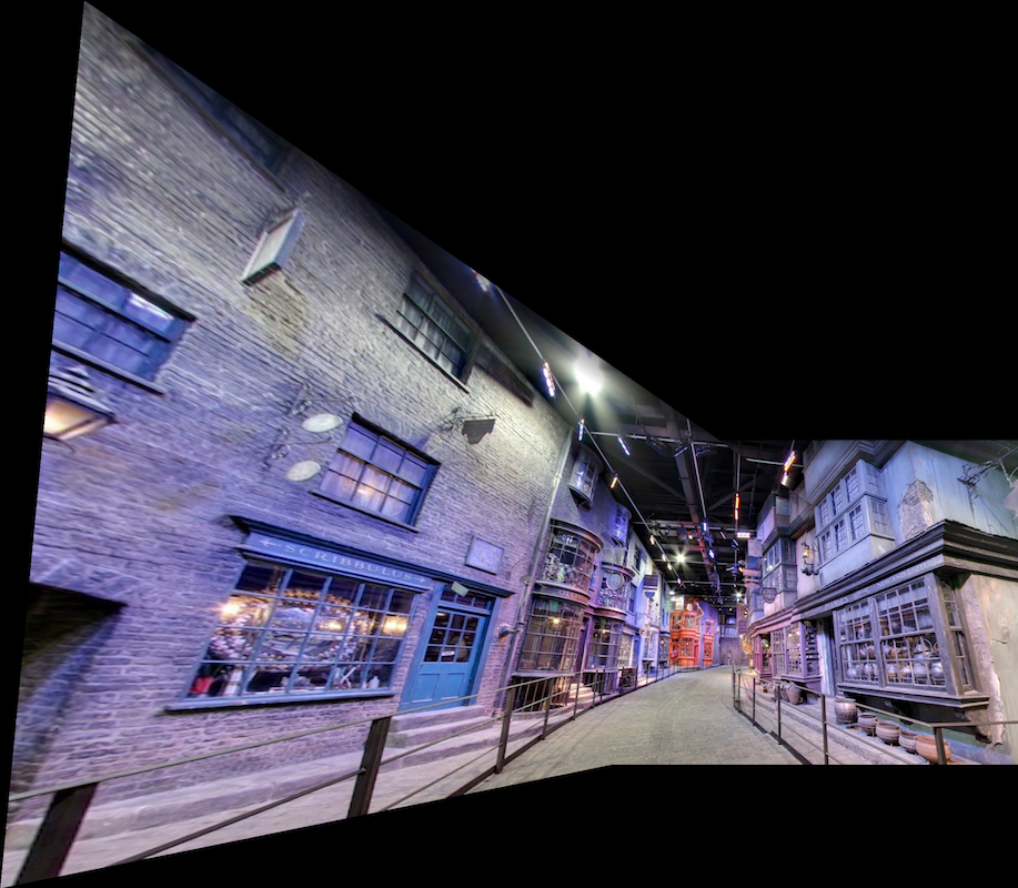
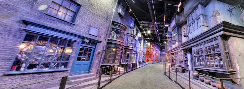
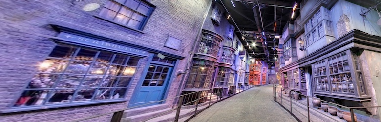
Harry Potter Studio
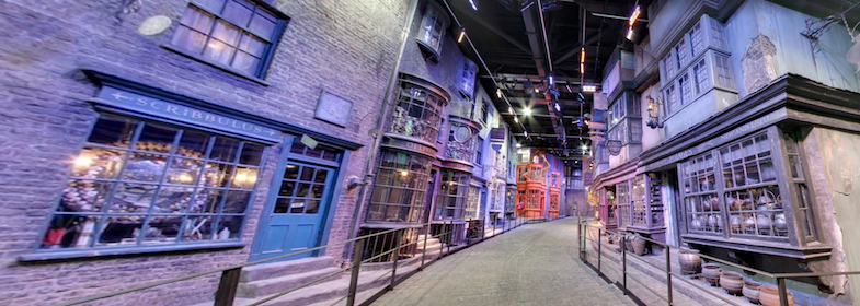 |
|---|
Cropped Result |
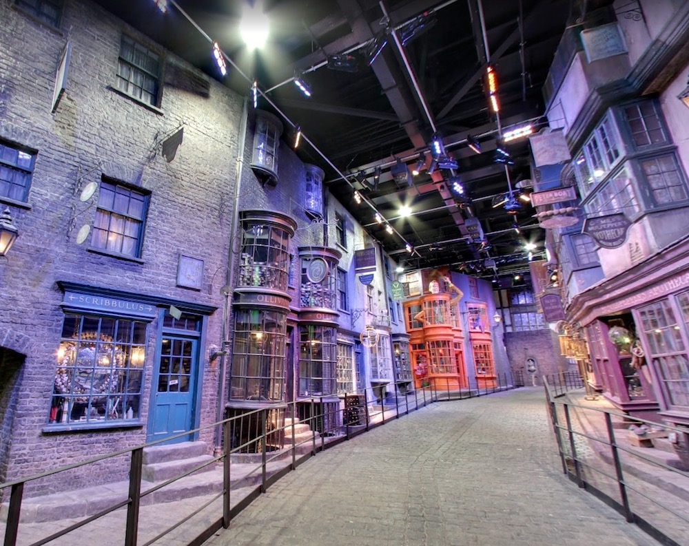 |
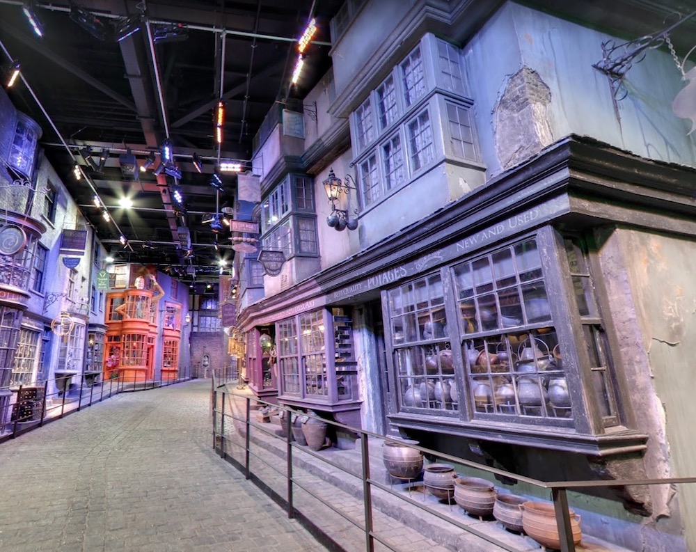 |
 |
|---|---|---|
| Left | Right | Blended |
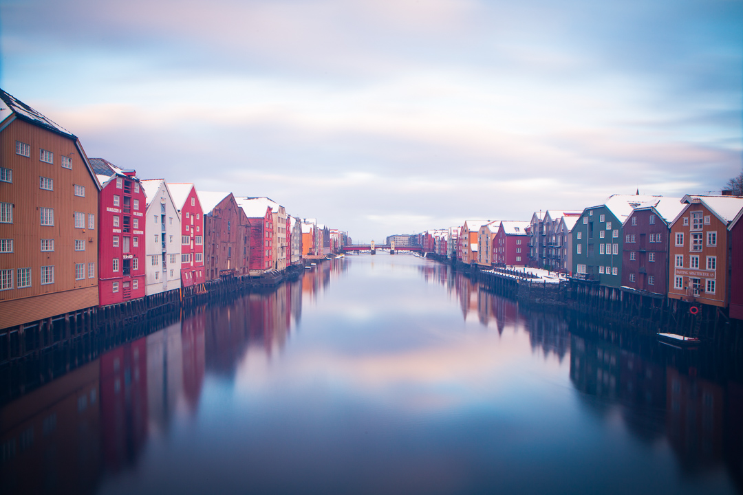
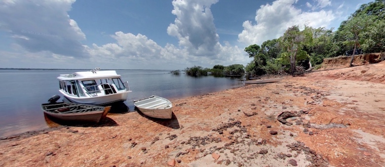
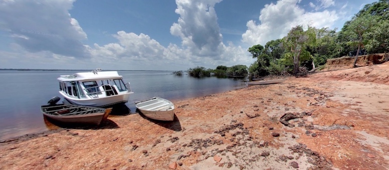
Saracá Dock
 |
|---|
Cropped Result |
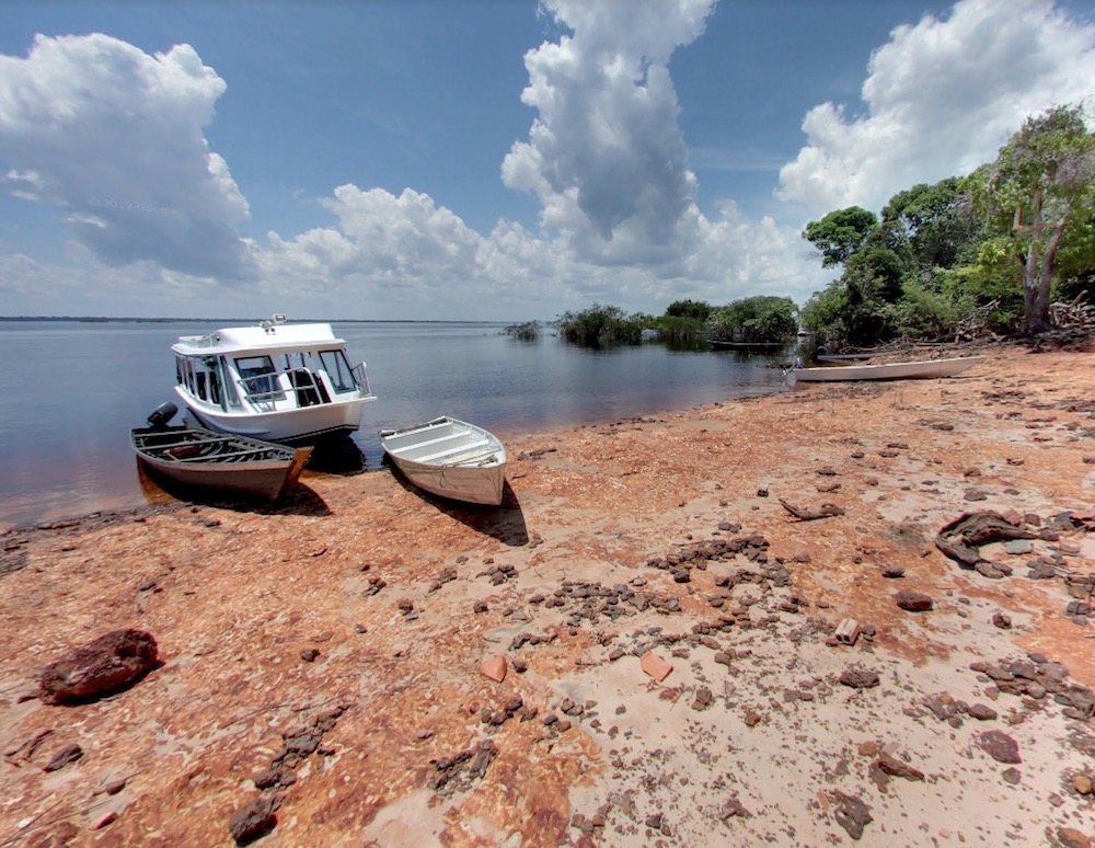 |
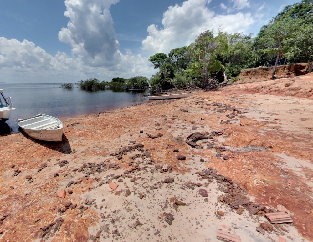 |
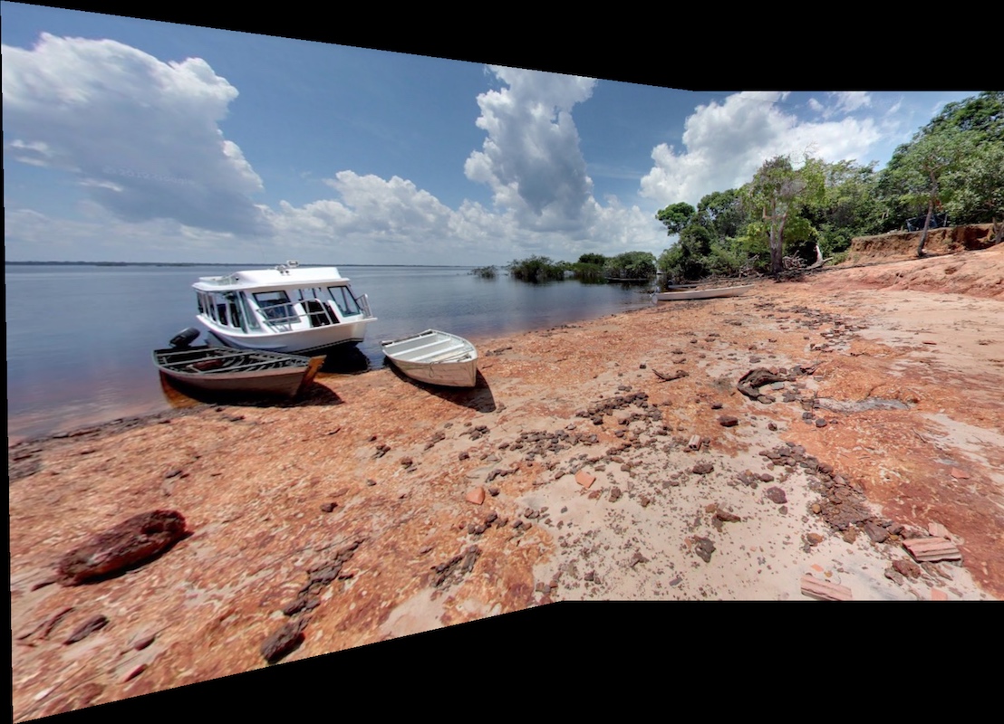 |
|---|---|---|
| Left | Right | Blended |
3 Feature Matching and Automatic Stitching
3.1 Theories
3.1.1 Harris Corners
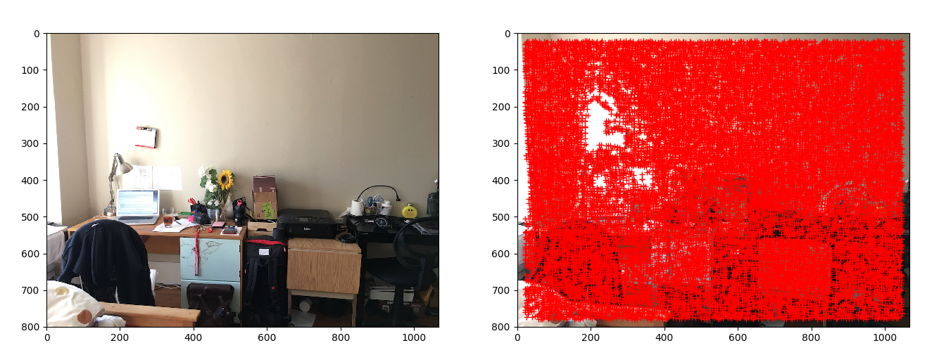
To detect similar features in a pair of images, we need a way to find correspondences between two images. I employed Harris Corners for this. Essentially, I scanned every single pixel, for every pixel location, I computed the R value which indicates how strong of a Harris Corner is at that location. Then I set a threshold to filtered out some weak corners.
 |
|---|
Image overlaid with Harris Corners. |
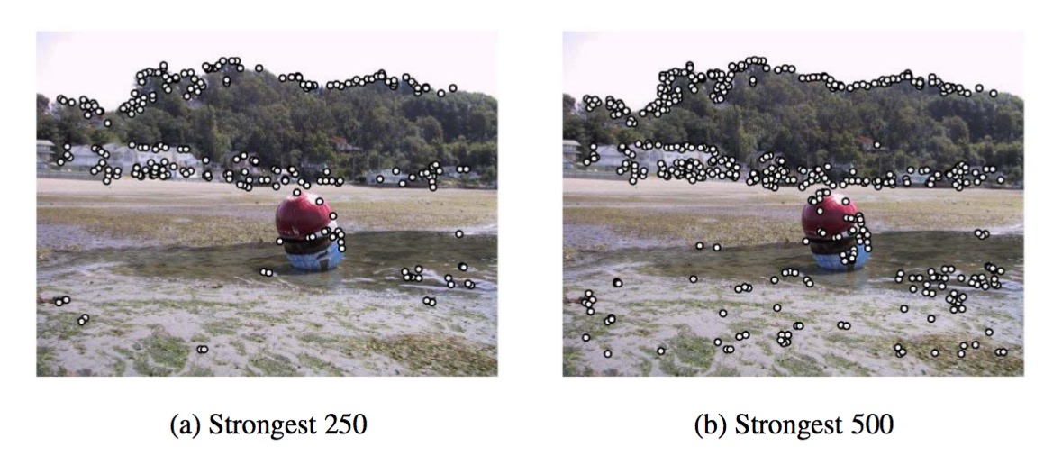
3.1.2 Adaptive Non-Maximal Suppression (ANMS)
From above we can see, we ended up over tens of thousands of corners. To further reduce this number, I implemented Adaptive Non-Maximal Suppression. One might ask why don't we simply set higher threshold to filter out more weak corners. This will result in clustering of points as shown in the following.
 |
|---|
Strong Harris Corners tends to cluster together. |
With ANMS , for every corner, we find the maximum radius r in which the point is the maximum (strongest) corner :
 |
|---|
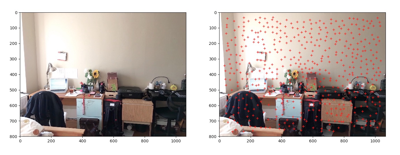
As suggested in the paper, I used c_robust= 0.9. That means that the radius r_i for point i is the minimum distance to a corner that is at least 1.1 times stronger than itself (0.9 is the discount factor. 0.9 discounted is the same as 1.1 times stronger). Once we have the radii for all corners, we sort them in descending order and pick the top 500. Below are the corners on the image after AMNS
 |
|---|
Top 500 corners with ANMS |
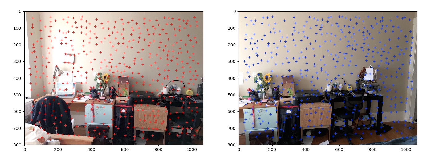
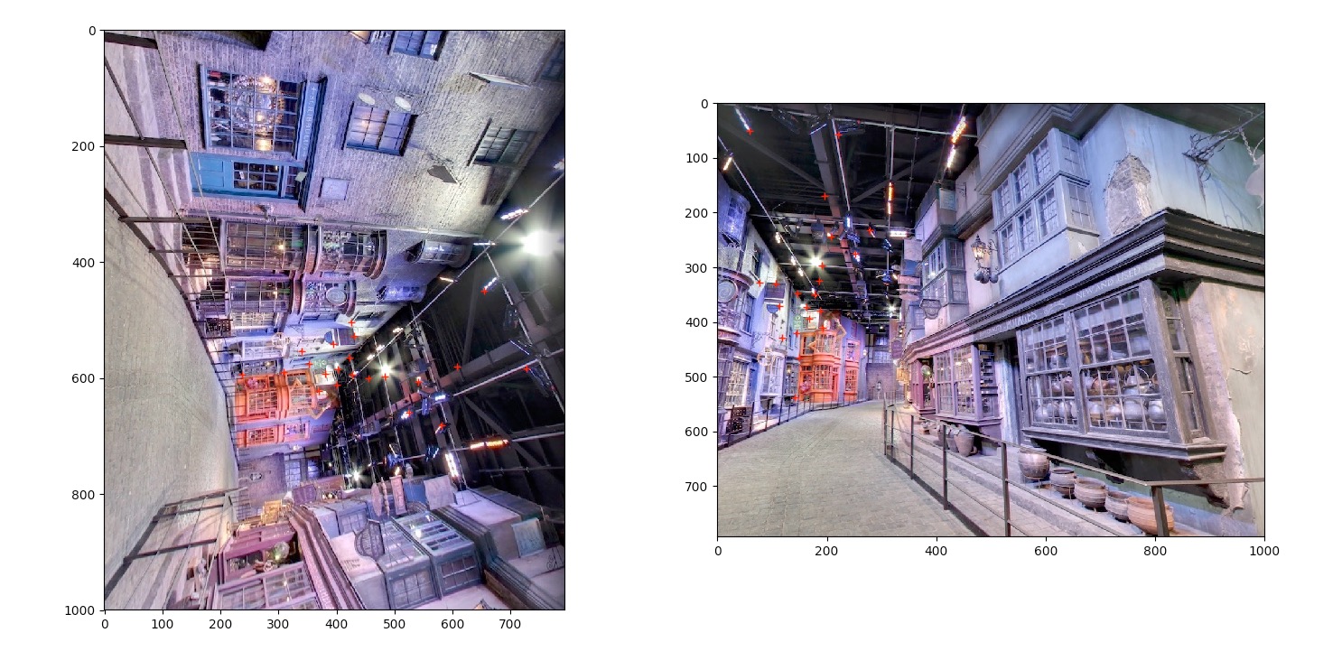
Now we put the two images side by side with ANMS top 500 corners.
 |
|---|
Top 500 corners with ANMS on both images |
3.1.3 Feature Descriptors
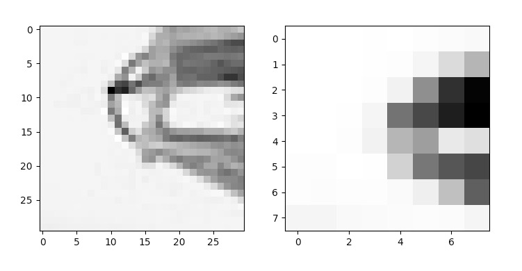
The first step is to find feature descriptor for each corner so that we can compare them in two images for finding matches. The basic idea is to compute a feature descriptor for each point from ANMS by sampling a 40 x 40 patch centred at each point, down-sampling to an 8 x 8 patch, and then normalising this patch by Z-scoring i.e. subtracting by the mean and dividing by the standard deviation s.t. it has mean 0 and sd 1.
However, this approach is not rotational invariant. So, on top of the basic ideas, I made the patches orientation invariant. Bear in mind that our goal is to find 8 x 8 orientation invariant patches.
Procedure
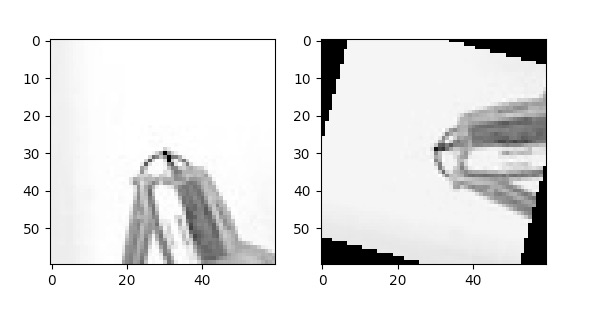
First for each corner location, we extract a 60 x 60 patch (bigger than 40 x 40 so that we can trim after rotation). Then we compute the Dominant direction of gradient from the centred 40 x 40 pixels. After that, we counter-rotate the patch so that they all face the same direction
 |
|---|
60 x 60 patches rotated to neutralised orientation |
After the 60 x 60 patch has been rotated to neutral position, I extracted the centre 40 x 40 pixels and then down-sampled it to 8 x 8 with Gaussian pyramid. Then, I z-scored all the patches so that they are invariant to lighting conditions. Finally, The patches are flattened into a 64-dimensional descriptor vector. Now regardless how the image is rotated and illuminated, all the patches will end up the same.
 |
|---|
60 x 60 pixel cropped to 40 x 40 then down-sampled to 8 x 8 using Gaussian pyramid. |
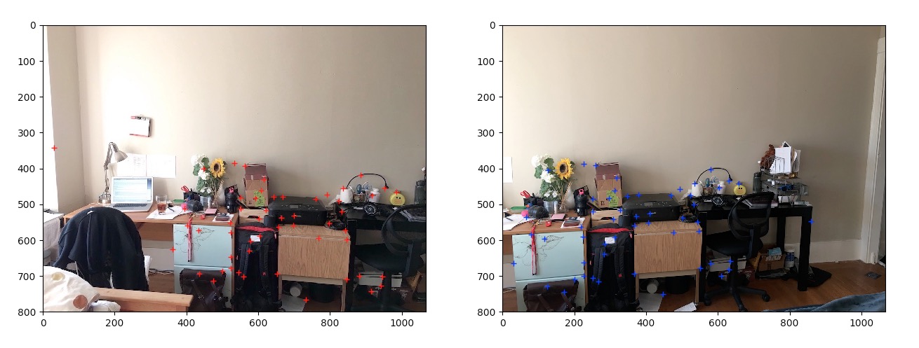
3.1.4 Feature Descriptors Matching
Now we match each of the 500 corners in the first image with those in the second image. We compute the SSD of each pair of corners. The next step is to match descriptors from im1 to im2, meaning we match a corner from im1 to a corner in im2. We go through all the descriptors from im1, and find the closest match in im2. The metric used is simply the SSD between the two descriptors.
To ensure that the best match is indeed the best match out of all corners in im2, we also consider the second closest match. If (SSD 1NN)/(SSD 2NN) is less than a threshold, then the first nearest match is indeed the best match. The threshold used is 0.35, as suggested by the paper. The insight behind is the the SSD of inlier should be statistically significantly higher then the SSD of outliers. This throws out most corners and keeps only those that have a (almost certain) match across the two images. Notice the matches are almost perfect except the points that doesn't exist in the other image.
 |
|---|
Remaining Corners after feature matching. |
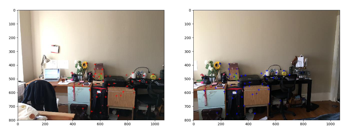
3.1.5 Random Sample Consensus (RANSAC)
RANSAC is a very robust algorithm to rule out outliers. To remove all the outliers and to compute a robust homography, we use 4-point RANSAC algorithm. We randomly select 4 'matching points' and compute H using only these four points. We then count the total number of inlier, where a point is considered an inlier if SSD(Hp, p') is less than a threshold, set to 1. We repeat this for a large number of iterations (in my case 1000 is beyond sufficient). After all the iterations, we keep the largest set of inlier including the 4 selected points and dump out all other points. The result is perfectly matched correspondences as shown below.
 |
|---|
Every point has a perfect match. |
Finally, we re-compute H using least squares on all the inlier. Once we have H, we apply the same warping and blending algorithms used in the first part of this project and obtain panoramas.
3.2 Results
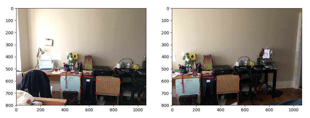
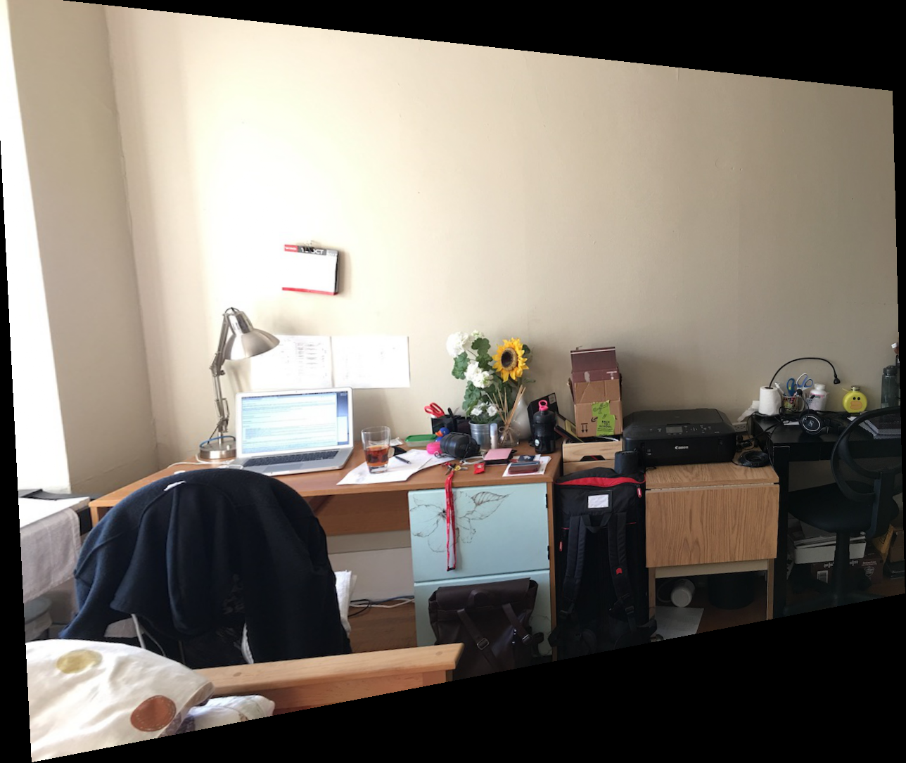
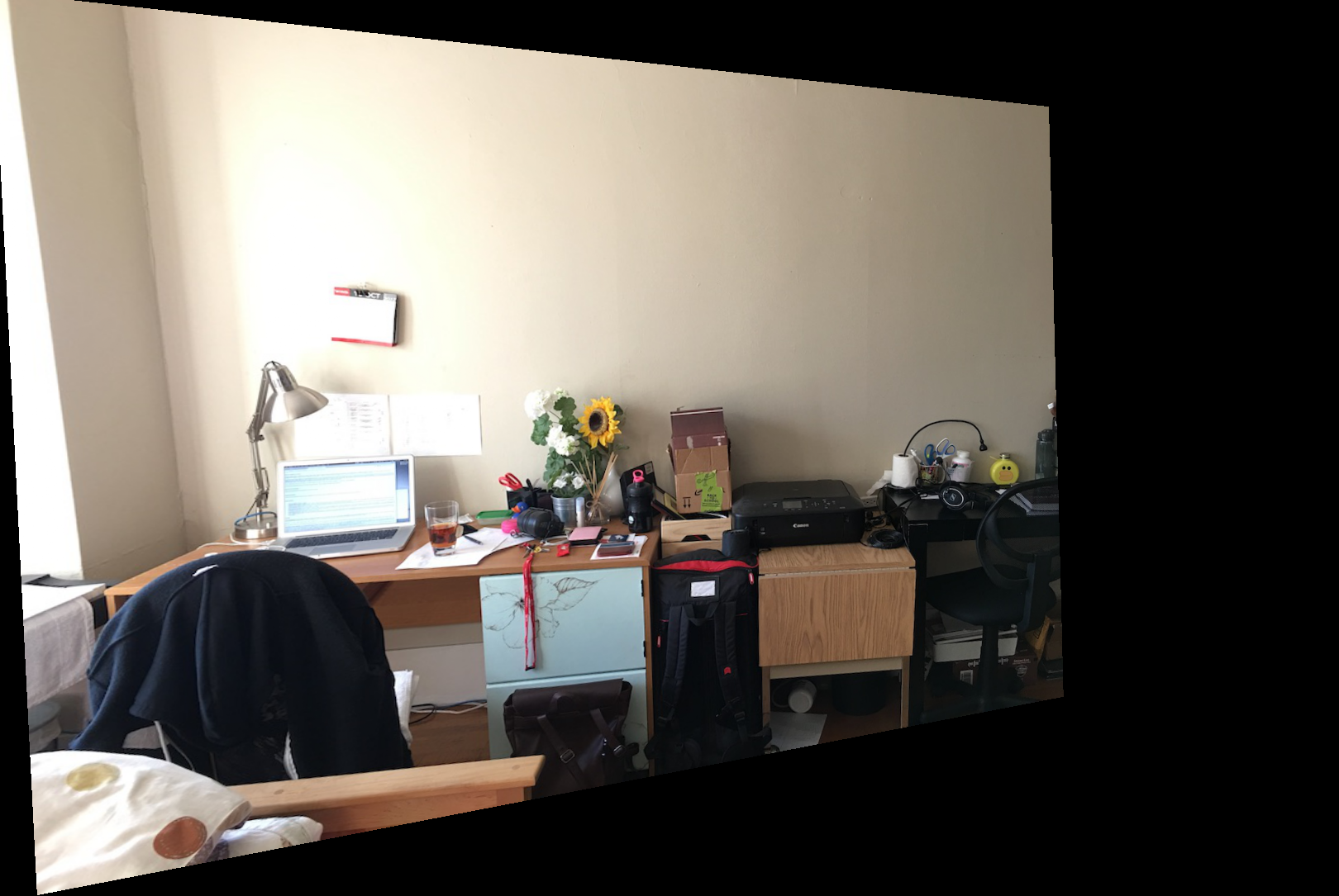
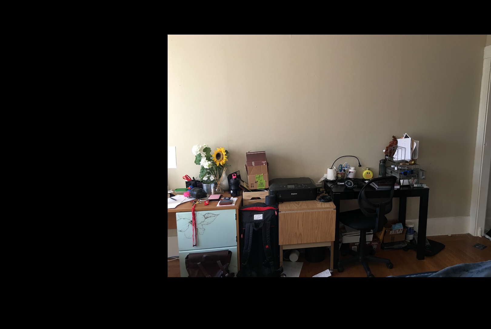
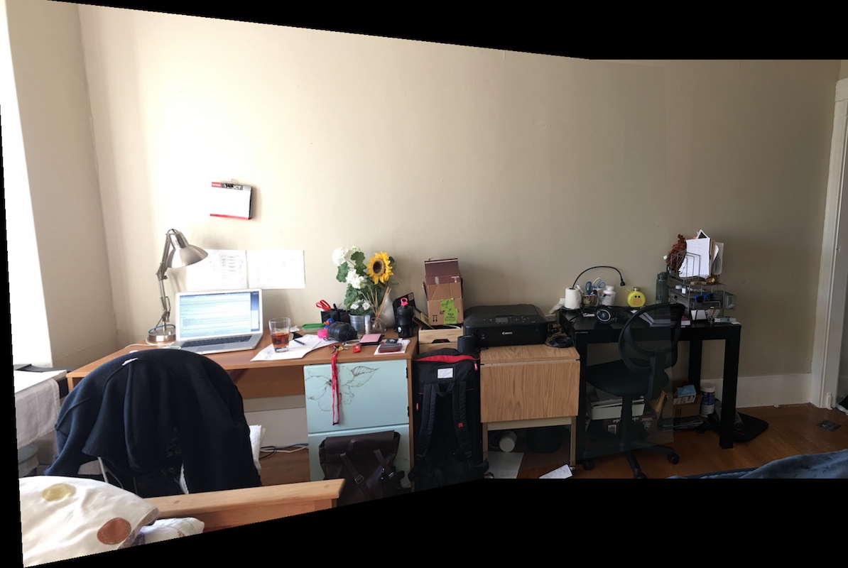
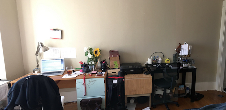
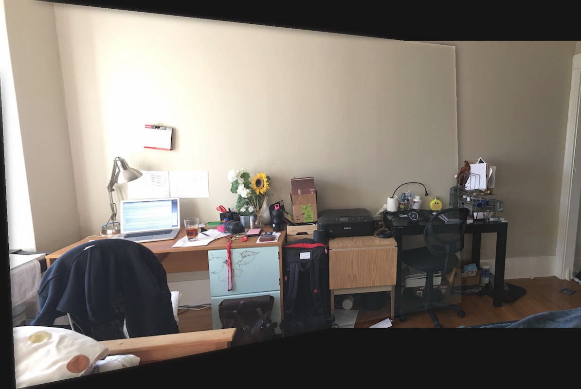
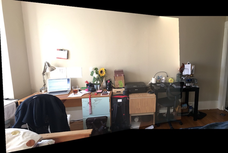
Room
 |
|---|
Manual |
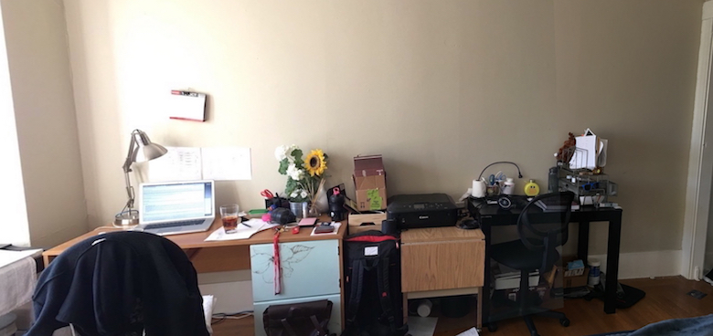 |
Automatic |
Harry Potter Studio
 |
|---|
Manual |
 |
Automatic |
Saracá Dock
 |
|---|
Manual |
 |
Automatic |
4 Bells & Whistles
4.1 Different Blending Techniques
 |
 |
 |
|---|---|---|
| α blending | Multi-resolution Gradient Domain Blending | Poisson Blending |
4.2 Rotational Invariant Harris Corners
Refer 3.1.3 above for detailed theory and implementation
 |
|---|
Perfect Correspondence match even though image has been rotated. |