In this project, we got to play around with image warping and mosaicing. In this part we got to play with cool concepts such as homography mapping between two images, warping one image into the shape of another based on key feature detections, and actually blending and stiching images together.
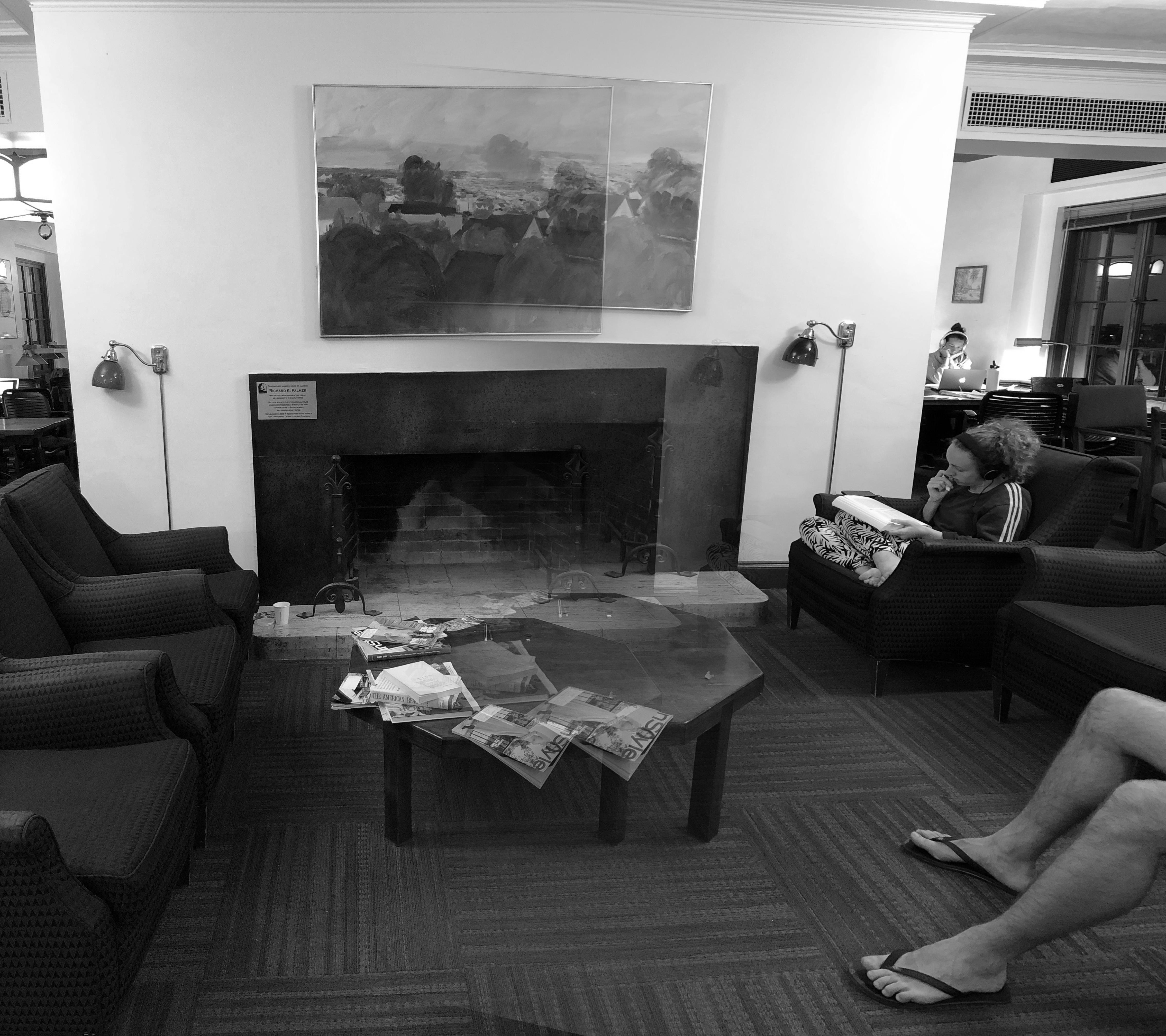
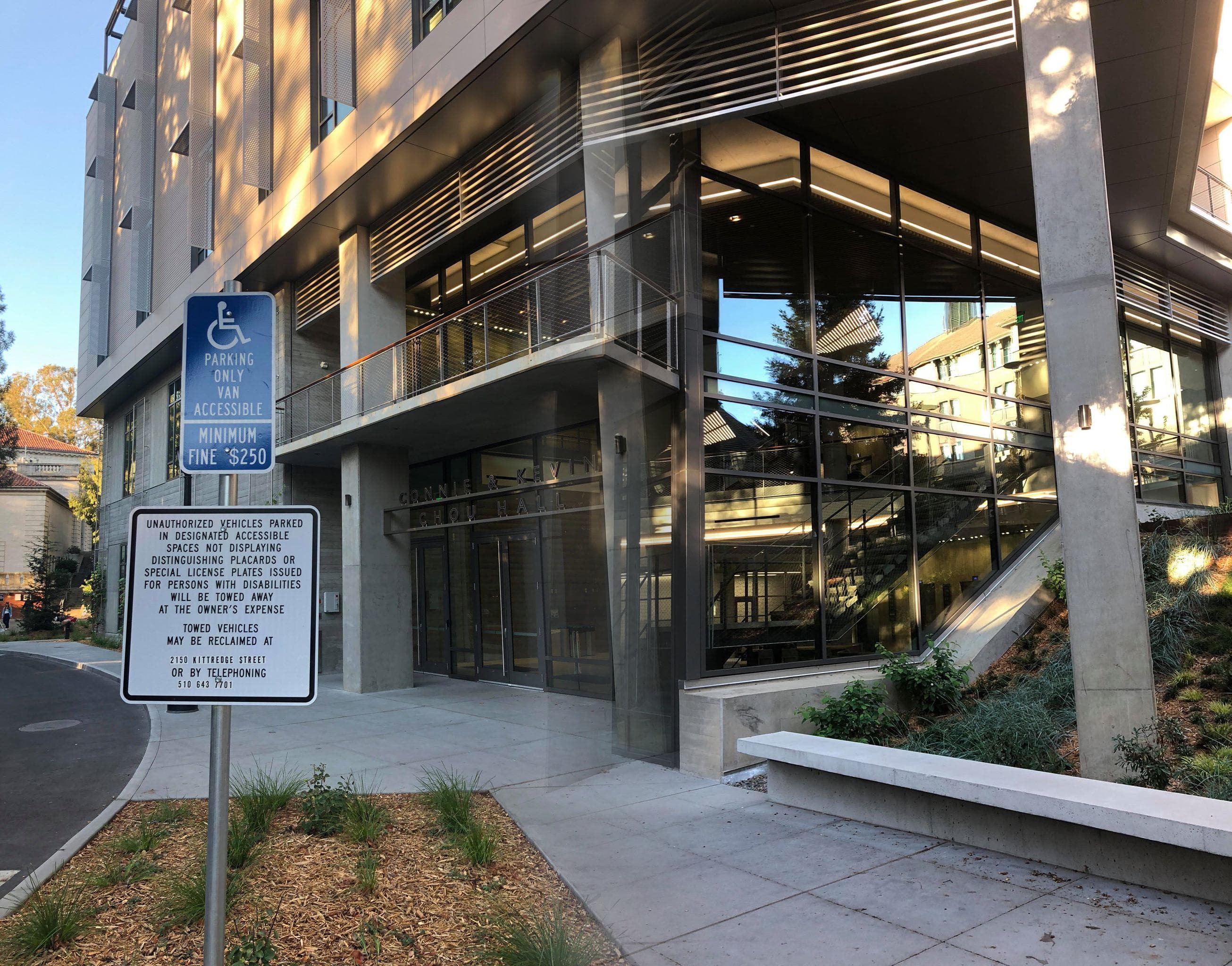
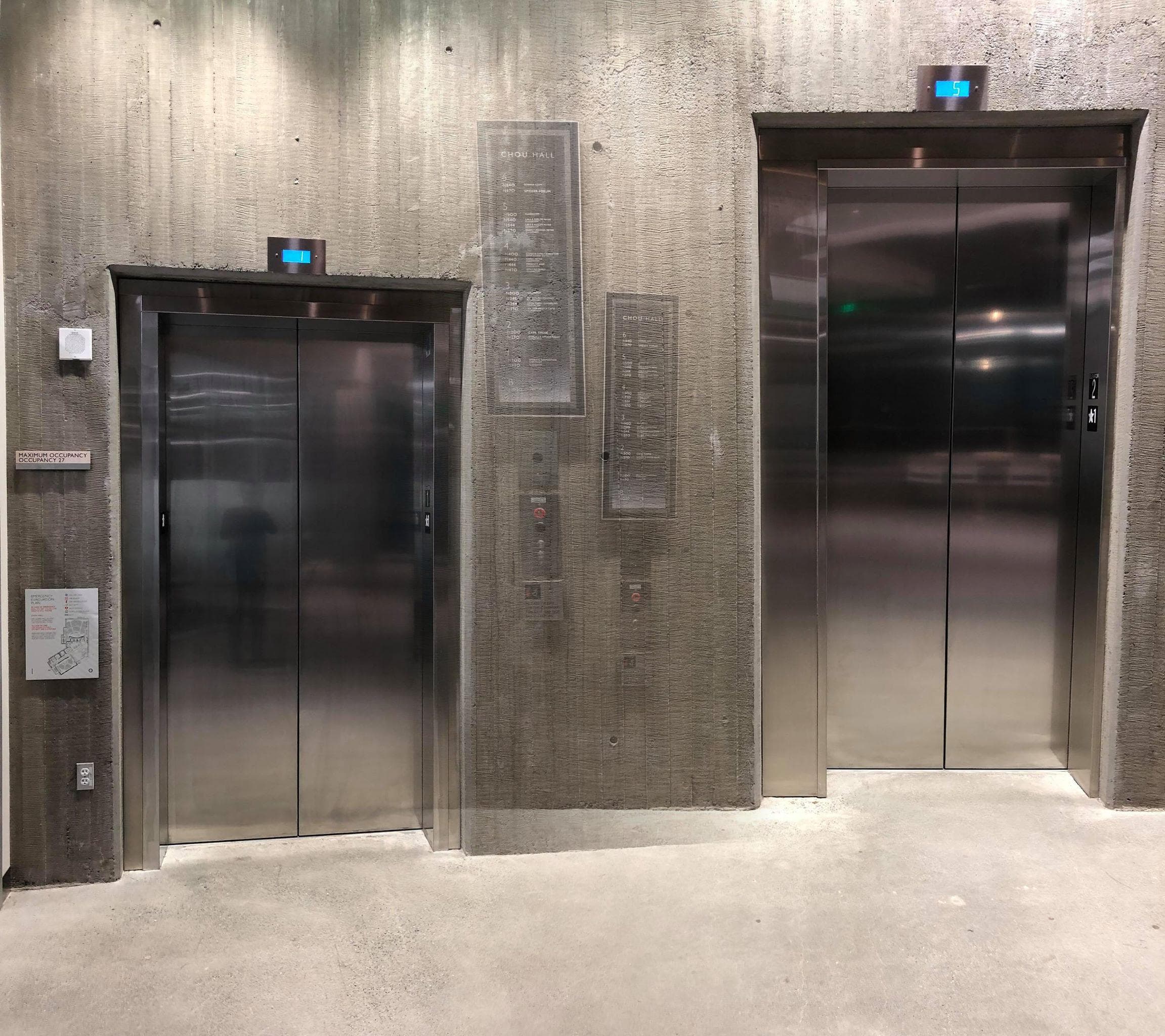
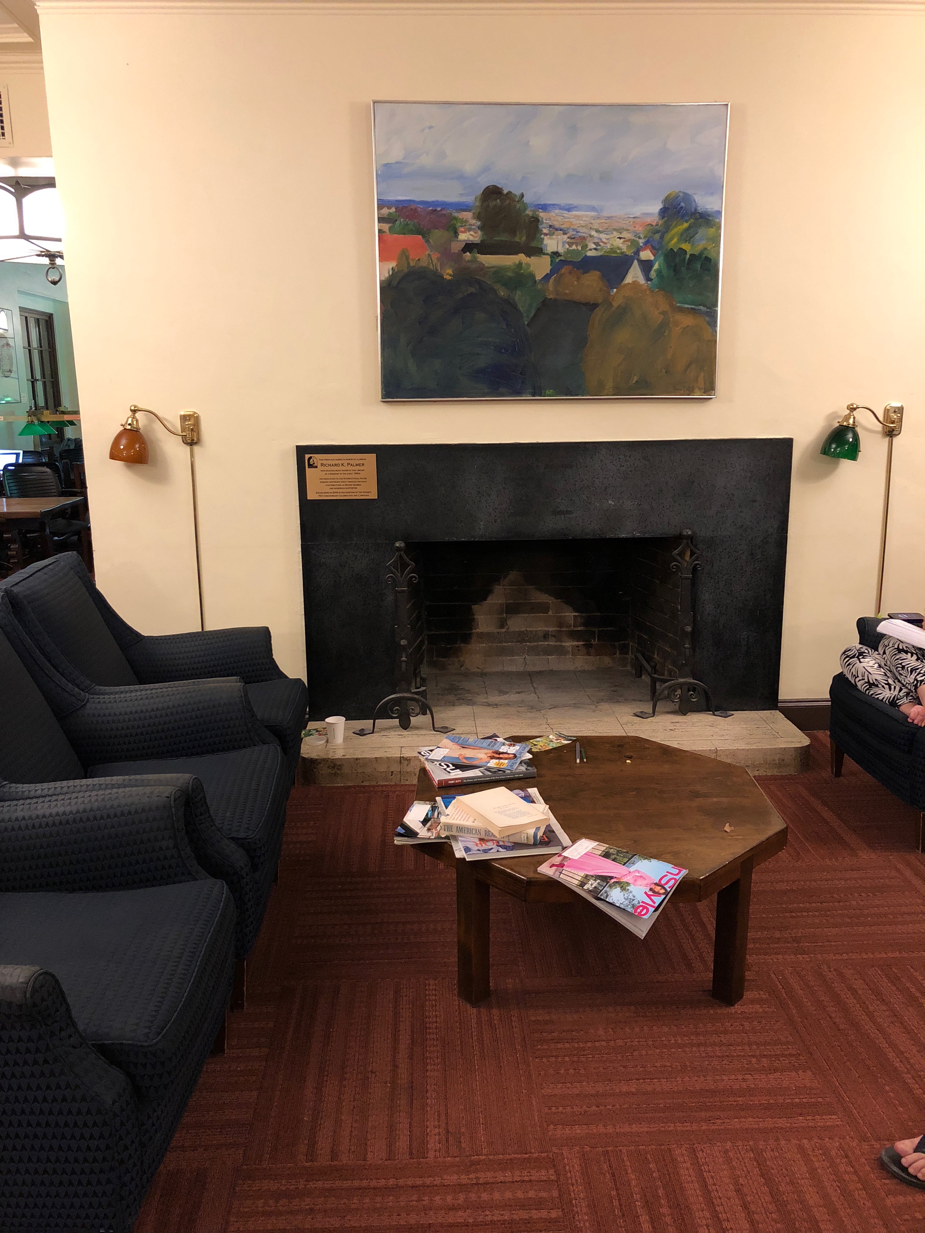
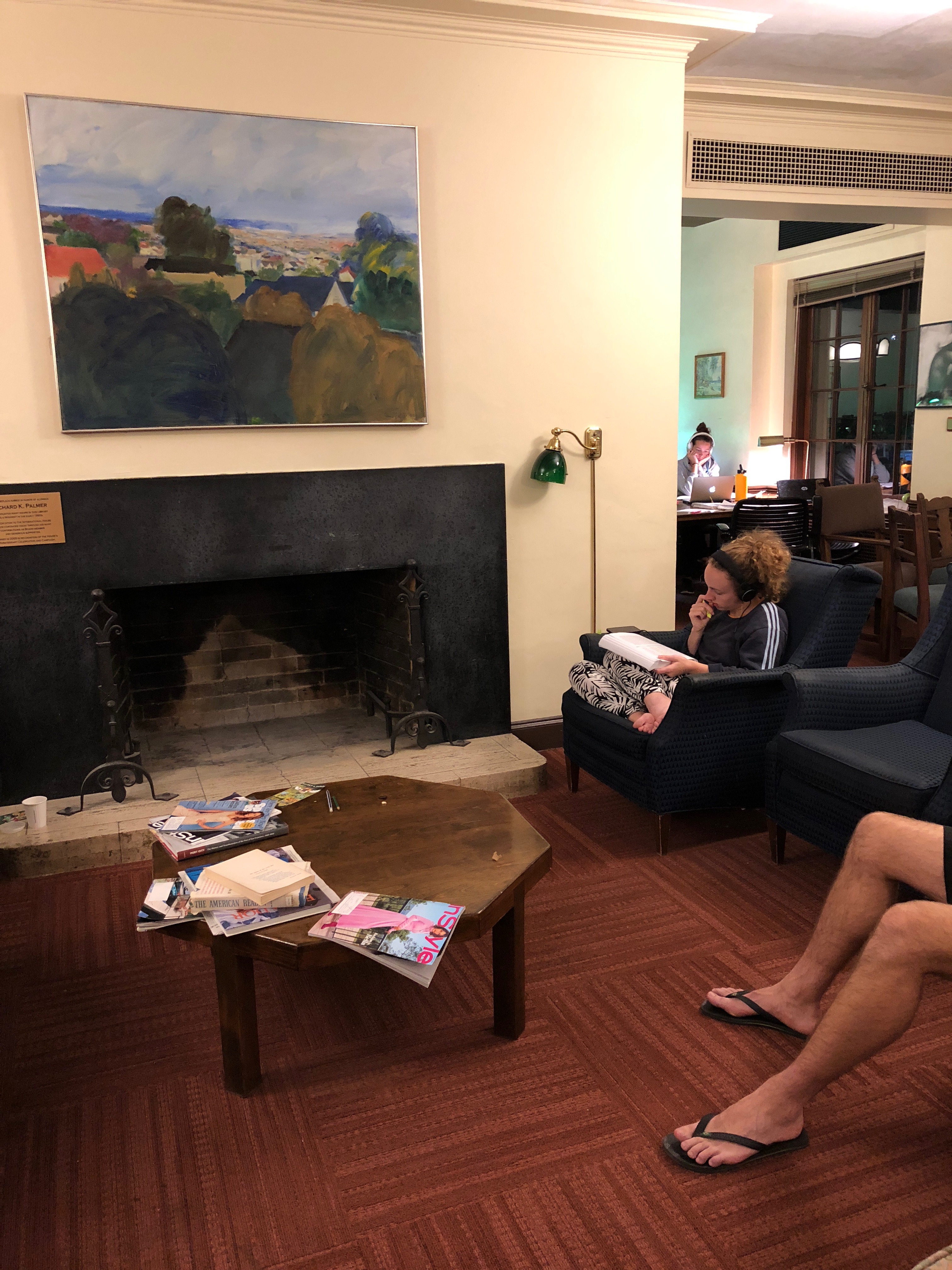
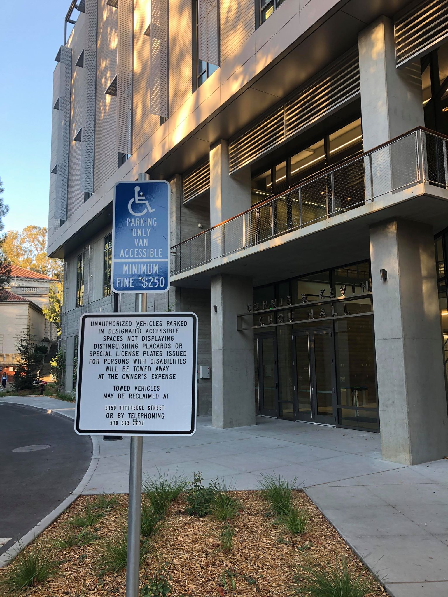
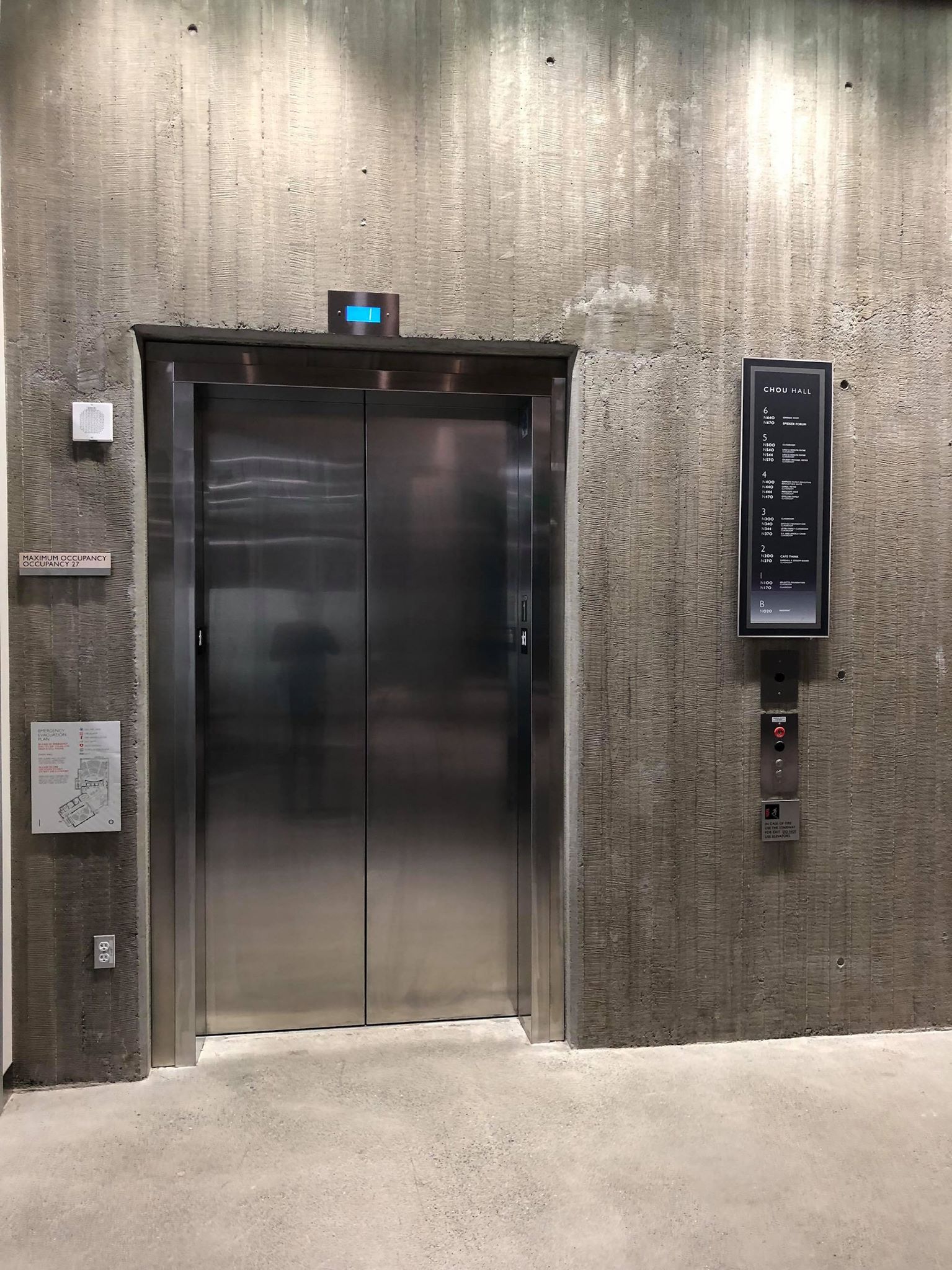
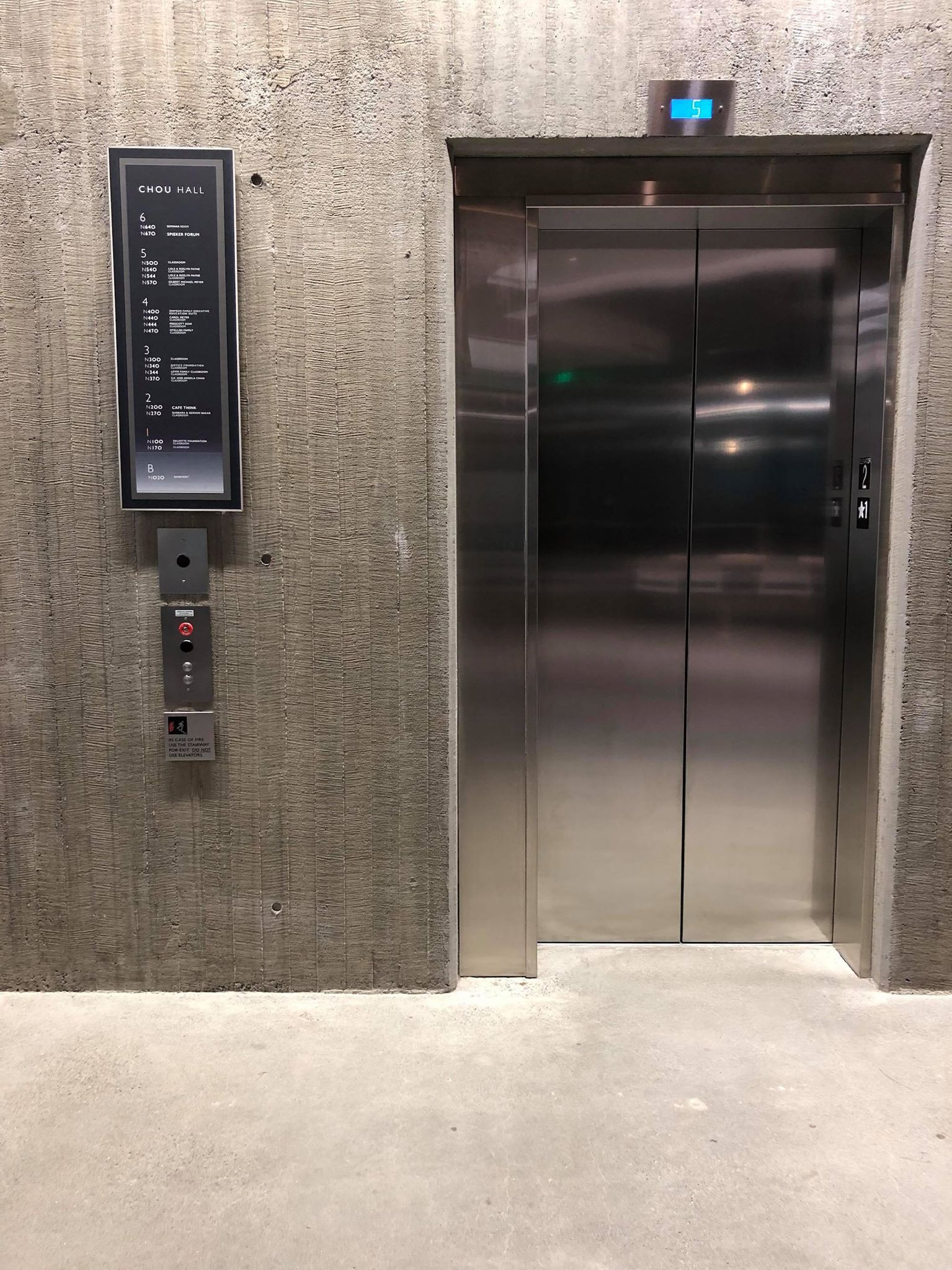
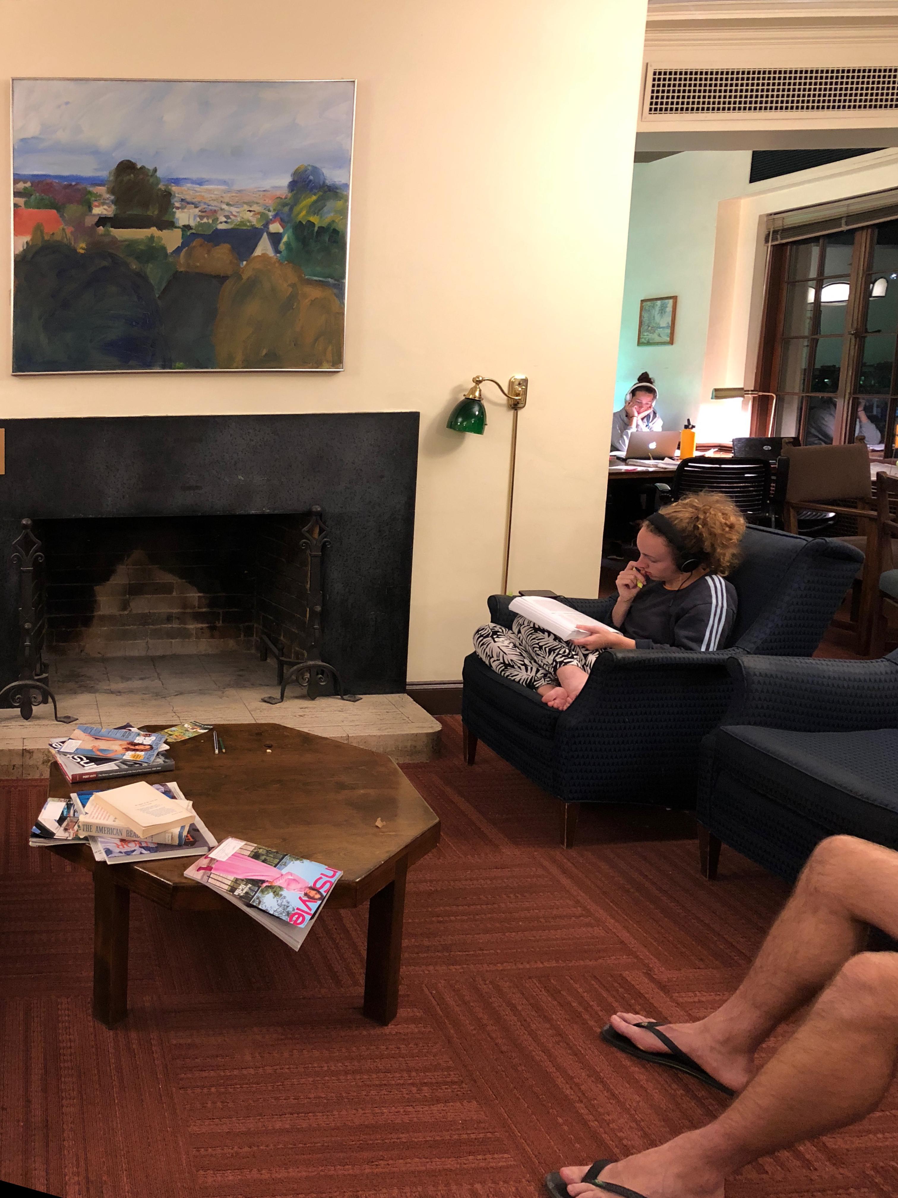
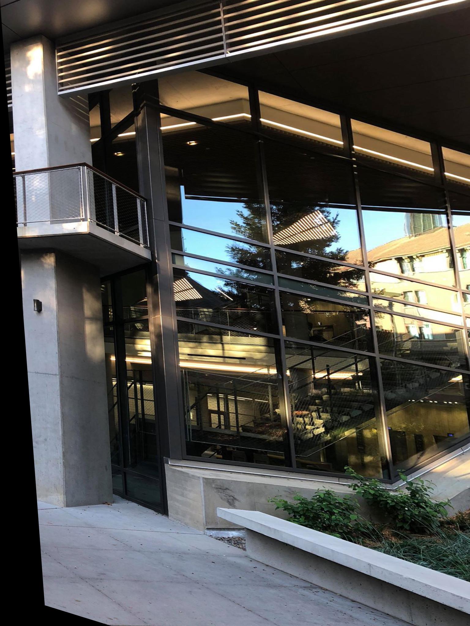
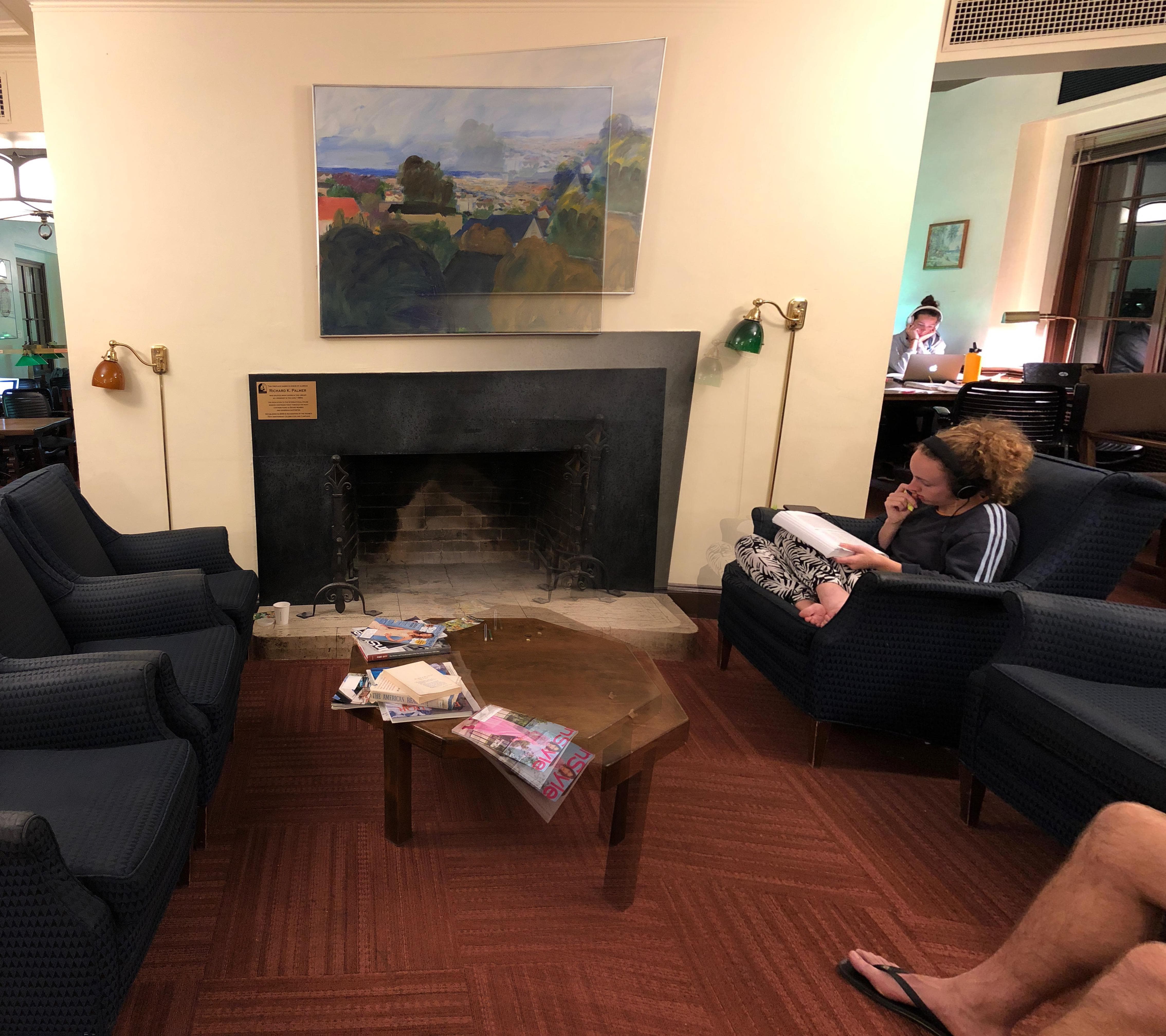
Below are all the pictures I used to create my different mosaics. These includes photos from a classy library, outside the esteemed Haas Business School, and elevators found inside a random UC Berkeley building. The set of images that worked best for me were the images I happened to capture at the classy library.

Next we recover the homographies between two images. A homography is an 8 paraemter matrix that basically transforms an image to the geometry of another image. In order to solve for our homography, we need four seperate points from both images to recover the 8 missing values. Using the mathematics on piazza, we developed a robust equation to solve for the missing values for our homography. Please see the image and the steps below. The below equation is for only one point correspondence, we need a total of 8 rows for all four input points.
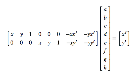
1. Create the left matrix using the input (x,y) values and the target (x', y') values.
2. Create the right matrix using the the target (x', y') values.
3. Depending on whether or not the left matrix is invertible, either use lin_alg.solve (if invertible) or lin_alg.lstsq (if not invertible) to recover the h vector.
4. Append the value 1 to the h vector, and then reshape it to be a 3x3 matrix!
Next we warp the images using inverse warping. The algorithm steps are below.
1. Calculate the warped images new top left corner points by applying the homography matrix to the original corner points.
2. Modify our homography matrix based on the new top left corner, and invert it.
3. Finally, use the inverted homography matrix to warp the photo.
Below are the original image and the warps I conducted. The first two warp/image rectification centers the painting from the classy library, the other warp/image rectification from haas centers the left most column.
Finally, I blended the images to create the different mosaiscs. The steps I used to create them are below.
1. Compute the homography matrix mapping image 2 feature points to image 1's feature points.
2. Warp image 2 to fit the geometry of image 1. Update image 2 to be this warped image.
3. Blend the aspects of image 1 and image 2 that overlap with each other. This changes depending on the images taken, but usually you blend the left half of image 1 and the right half of image 2.
4. Create the final stiched image that encompasses aspects of the first image, the blended middle image, and aspects of the second image.
Below is the moasics created for three diferent scenes. One is the classy library, two is outside the Haas School of Business, and three is the elevator found in a random UC Berkeley building.


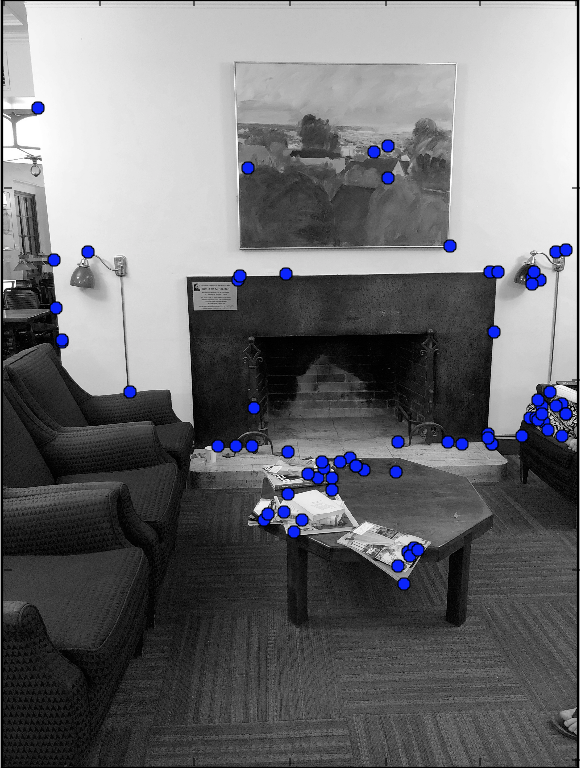
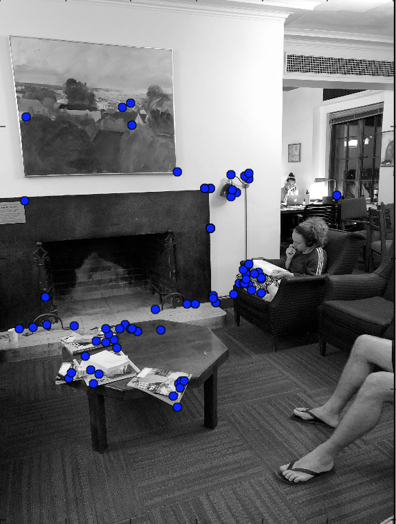
For part6B, we focused on autostiching the images together. We did through a series of steps including using harris corners, adapative non-maximal, suppression, feature descriptors, feature matching, and Random Sample Consensus algorithm. This part was really cool as we got to stich images together automatically that looked exactly the same, if not slightly better than the manually stitched ones!
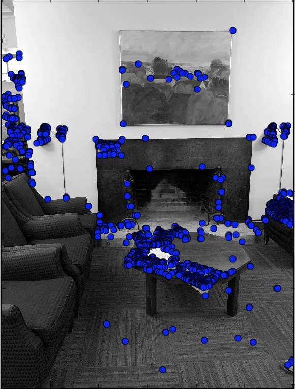
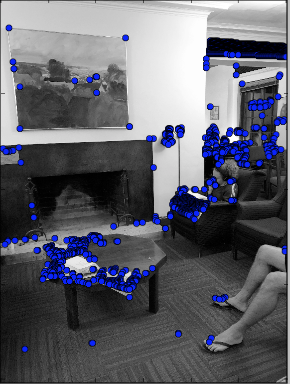
To detect the initial points we would consider when autostiching images together, we used the harris corner detection code given to us by Professor Efros. I made a slight edit and used corner_peaks instead of peak_local_max as advised by the GSI. This made the number of points selected go from 300,000 to about 1500! See the results below!
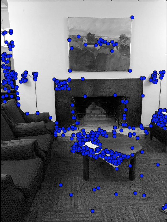
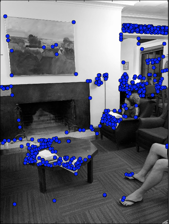
With over 1000 points to choose from, we need to find a way to filter them further. We do this through the anms algorithm as outlined in the MOPS paper. The algorithm is as follows:
Loop through all the harris points in a given image, and determine the minimum supression radius for each harris points as outlined in the algorithm in the MOPs paper: ri = minj|xi−xj|, s.t. h(xi) less than 0.9 * h(xj) where xi is a given harris point, xj is all other harris points, h(xi) is the intensity from the harris algorithm at thatb point.
For each harris point and minimum suppression radius pair, sort the outout such that we choose to keep the harris points with the 500 largest minimum supression radius.
Below are my results.
With now only 500 points, I needed to match the features found and both images together. First I needed to determine what those feature where and then actually match them.
To determine what those featurs where I first considered a 40x40 patch surronding a given anms point (determined previously). I then applied a Gaussian filter to this patch, scaled it down to an 8x8 patch, and normalized the patch. This gives an 8x8 feature descriptor for each anms point and makes it easier to match.
Below I have selected some random feature descriptors that I found from the 500 anms points.
With feature descriptors in hand from each image, I match the features together between both of the images. I do this using the Lowe algorithm in the MOPs paper and the dist2 method provided by Professor Efros. The algorithm is as follows:
1. For each feature descriptor in a given image, find the 1-NN (nearest neightbor using SSD) in the other image and the 2-NN (second nearest) in the other image.
2. If we can find a feature descriptor such that its 1-NN/2-NN is less than 0.3, then the feature descriptor in the given image and the 1-NN in the other image are see as matches.
3. I then return the points of the two feature descriptors (for the given and other image) above.
Below are my results.
The only thing left is to compute the homographies! We use this according to the RANSAC algorithm below:
1. Select four feature pairs and random between two images.
2. Compute homography between the given image and the other image by using these points as the correspondence. 3. Calcuate the distance between the other image points and the computed points from step 2, keep the points with an error less than 10 pixels. 4. Recompute the homography with the points that have that smallest error using least squares. See my final results below! The manually stiched image vs. the autostiched images. With some maybe minor nuances, the images look very similar to each other. It is super cool to see a program go about selecting images to stiching similar to how I do! I kept the auto-stiched classy library photo to be black and white since all my analysis above was black and white.