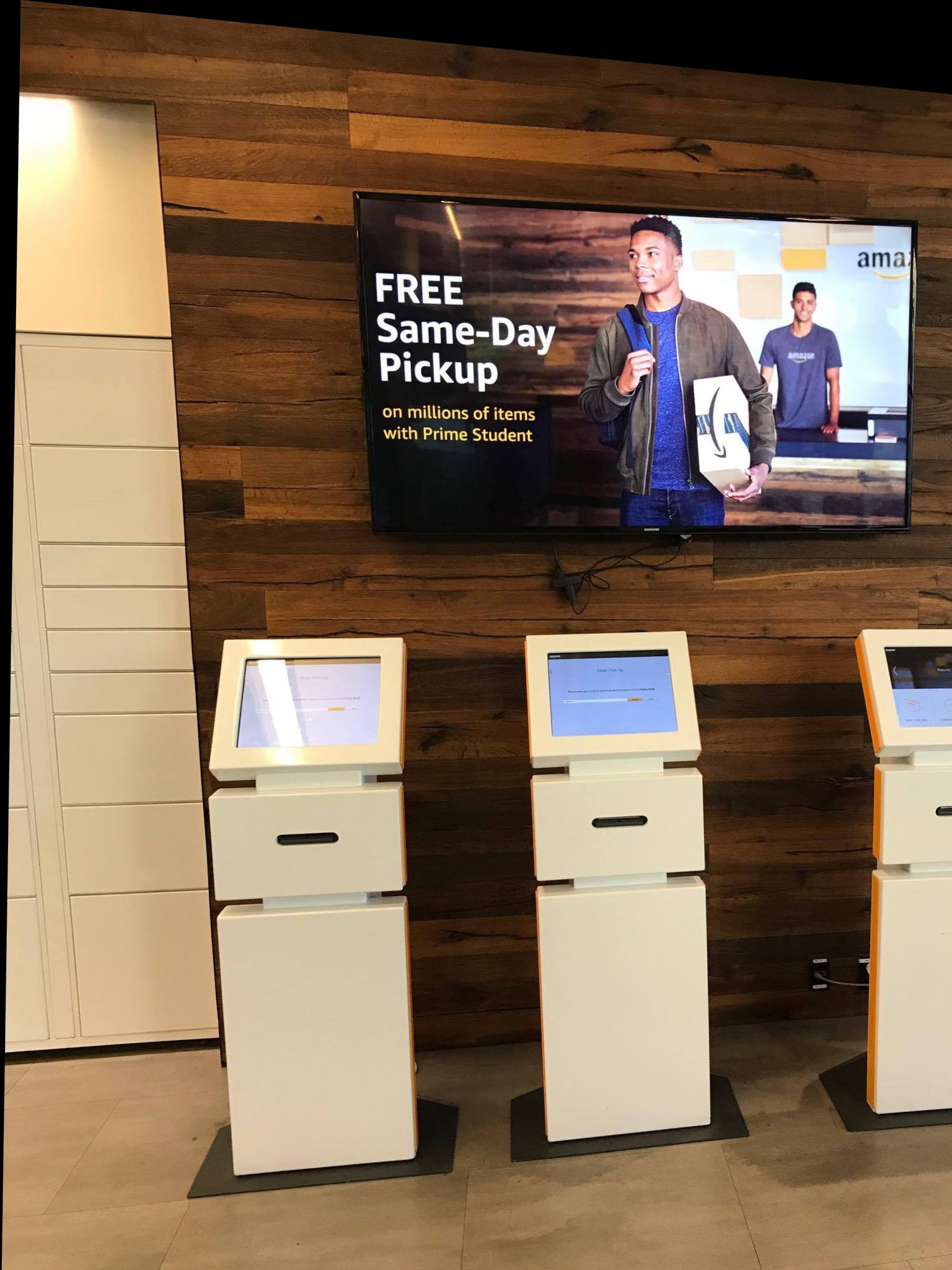
In this part we needed pictures to rectify and also create mosaics from. I have images I've taken at a variety of locations. I took pictures at MLK, International House, and International House Cafe. These photos that you can see below were taken with a I Phone.
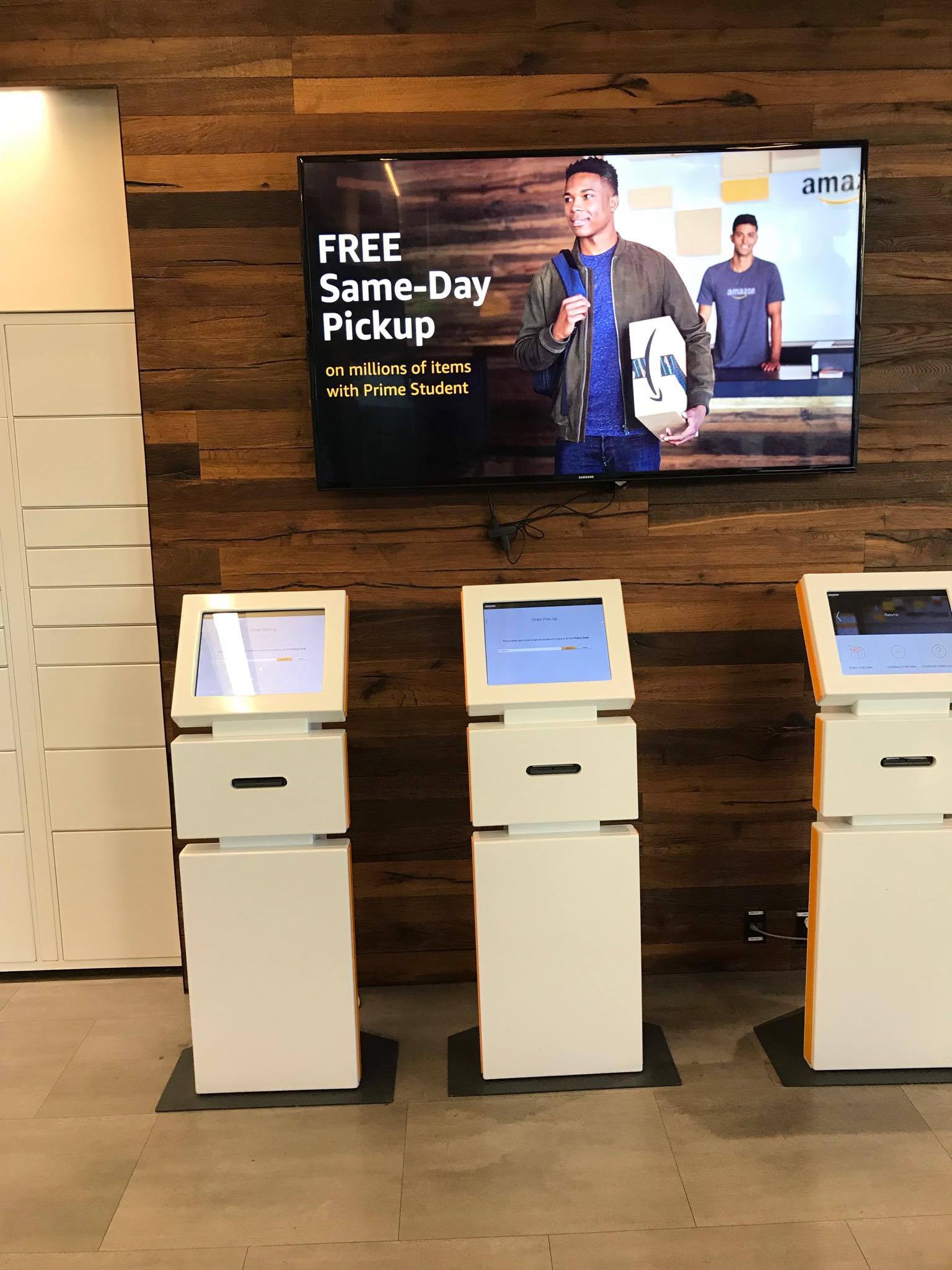
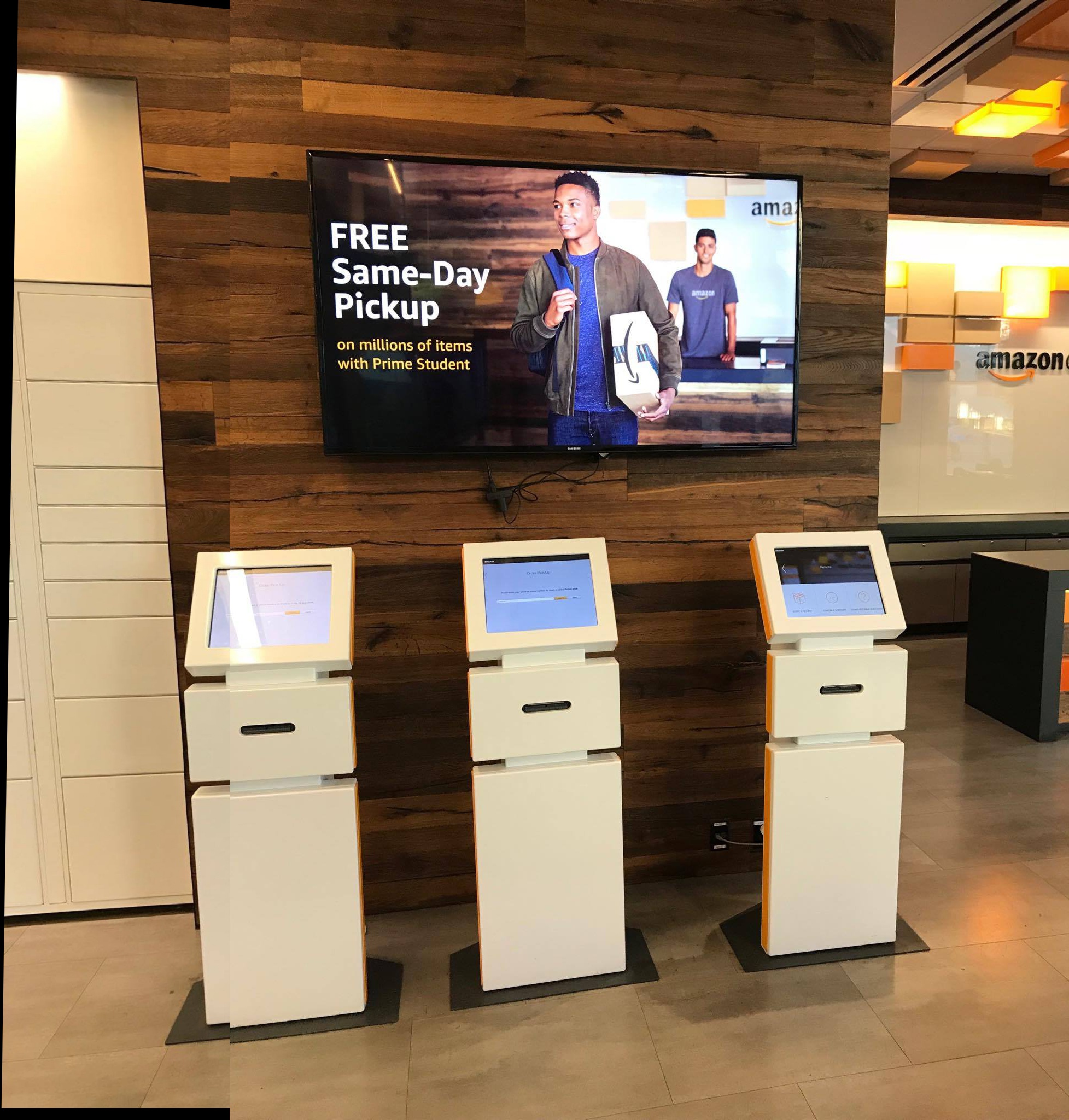
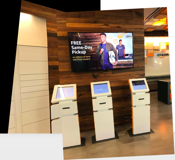
Left Image of MLK Amazon Store
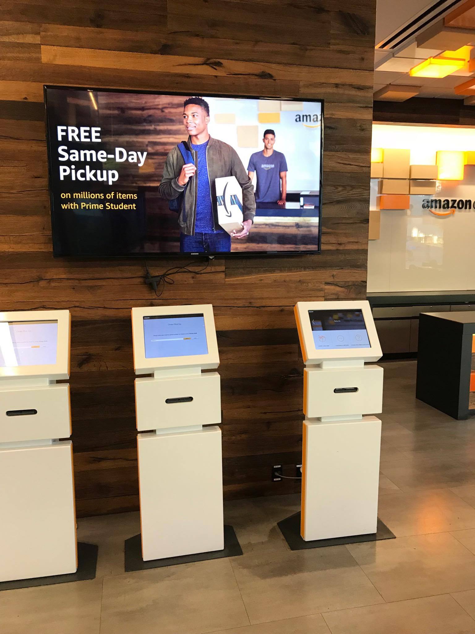
Right Image of MLK Amazon Store
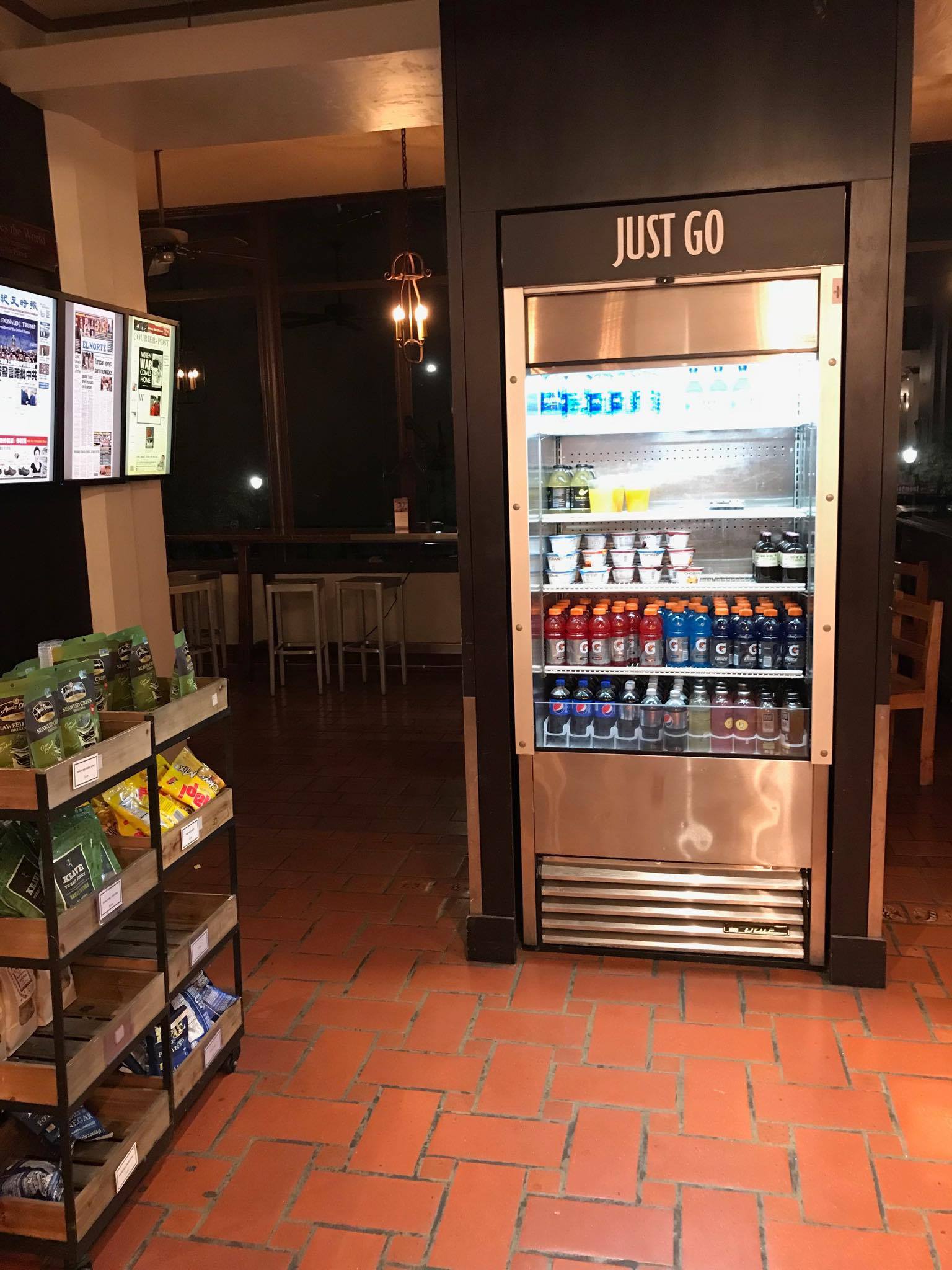
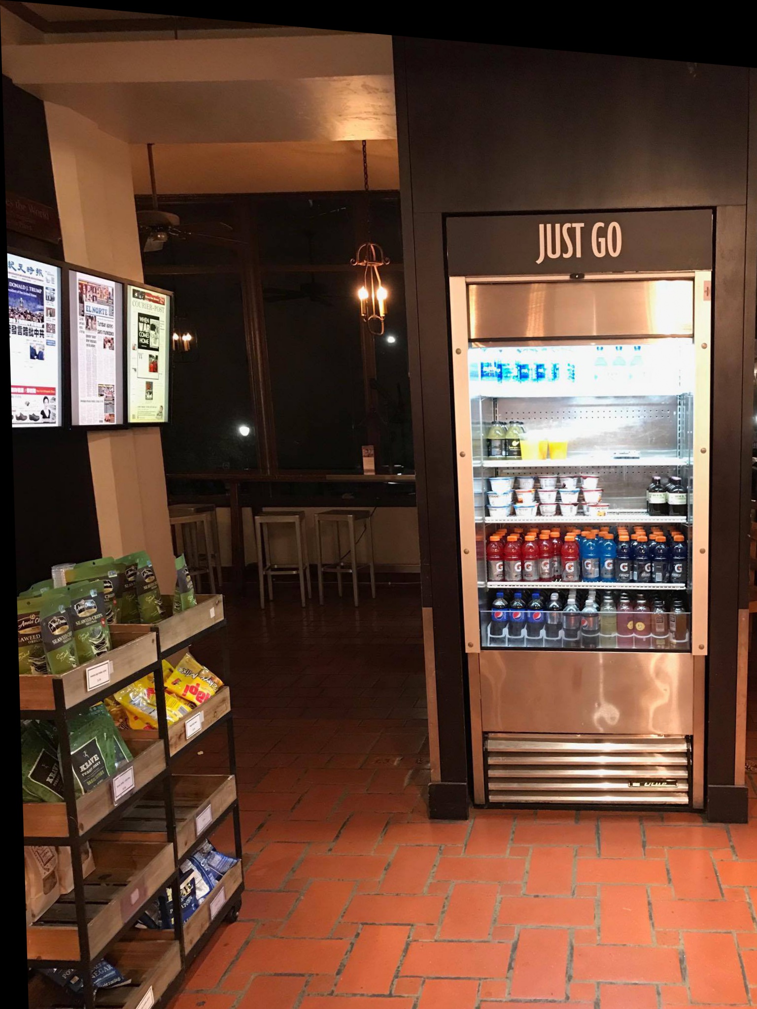
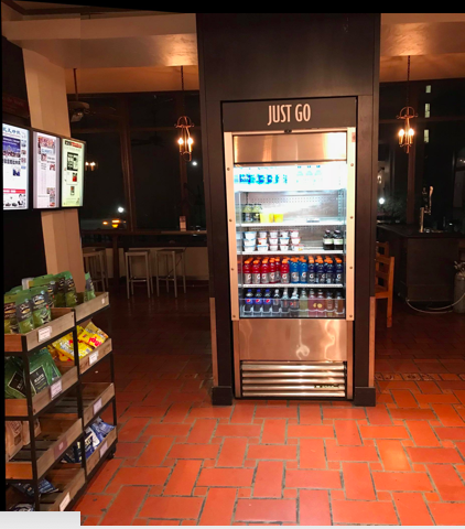
Left Image of ihouse cafe
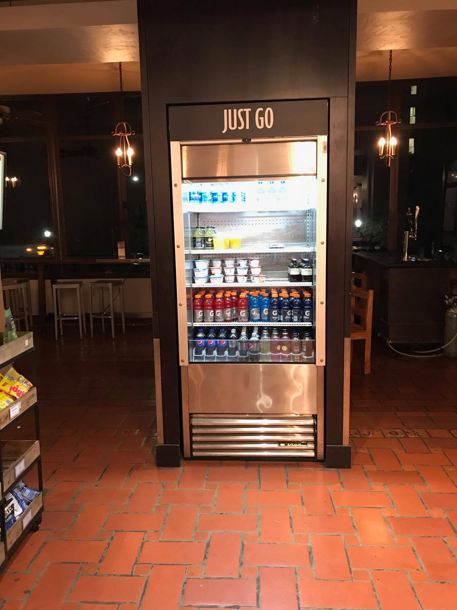
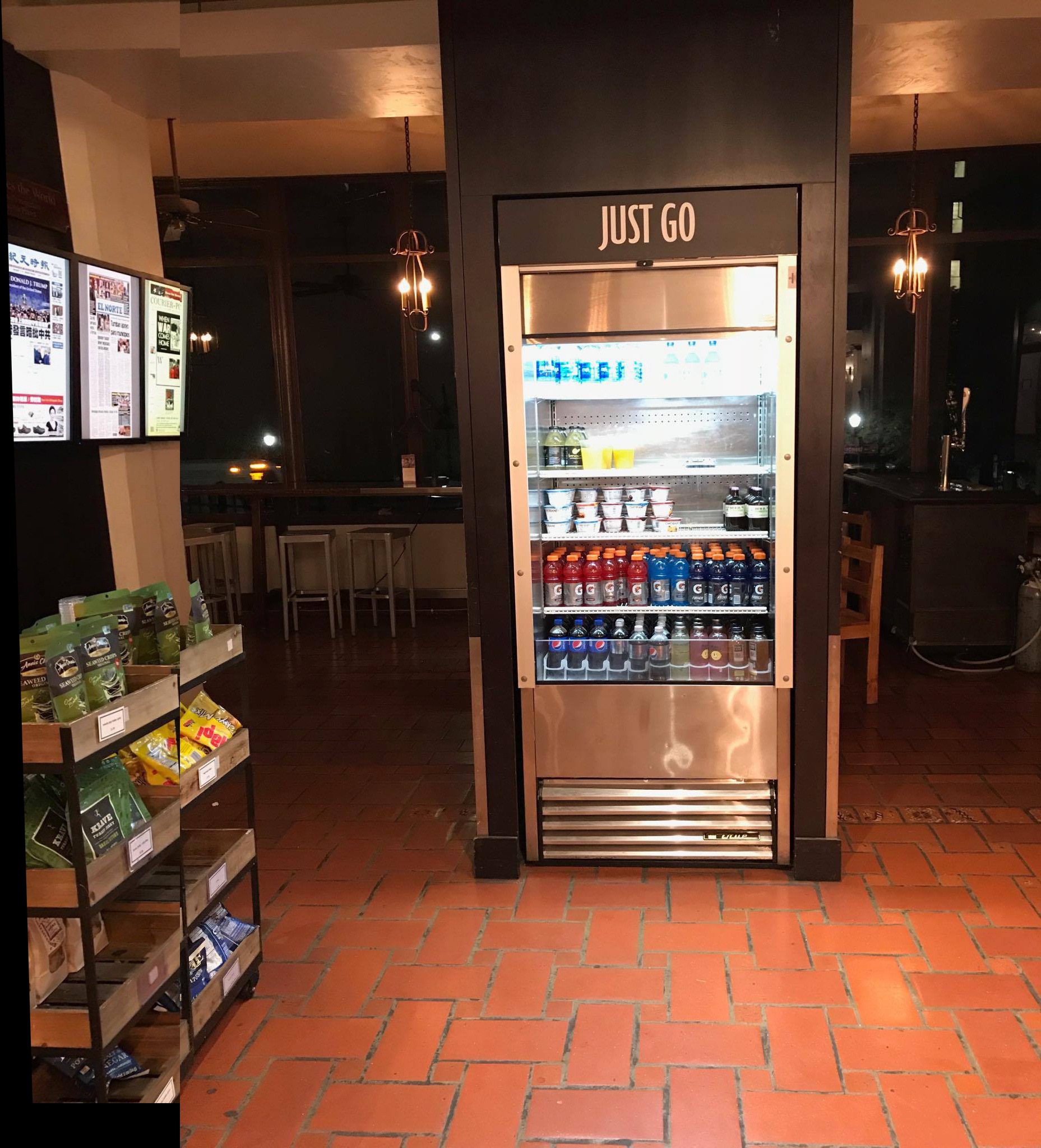
Right Image of ihouse cafe
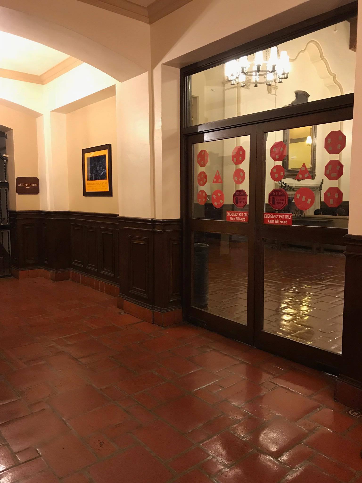
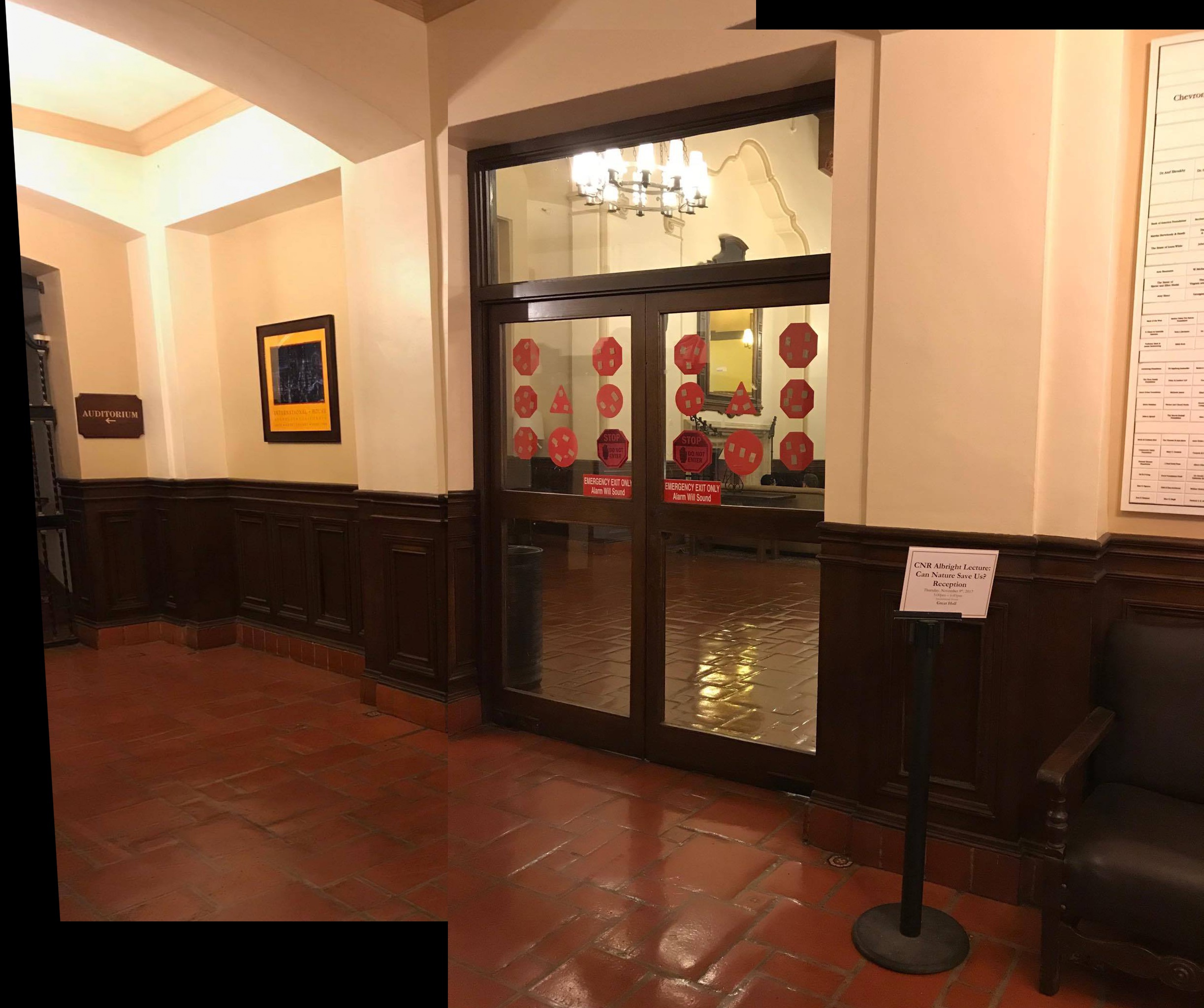
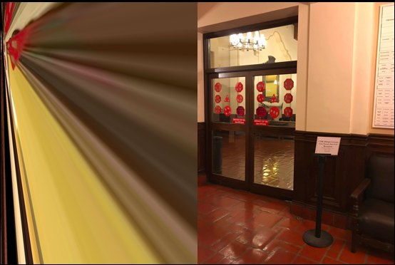
Left Image of ihouse door
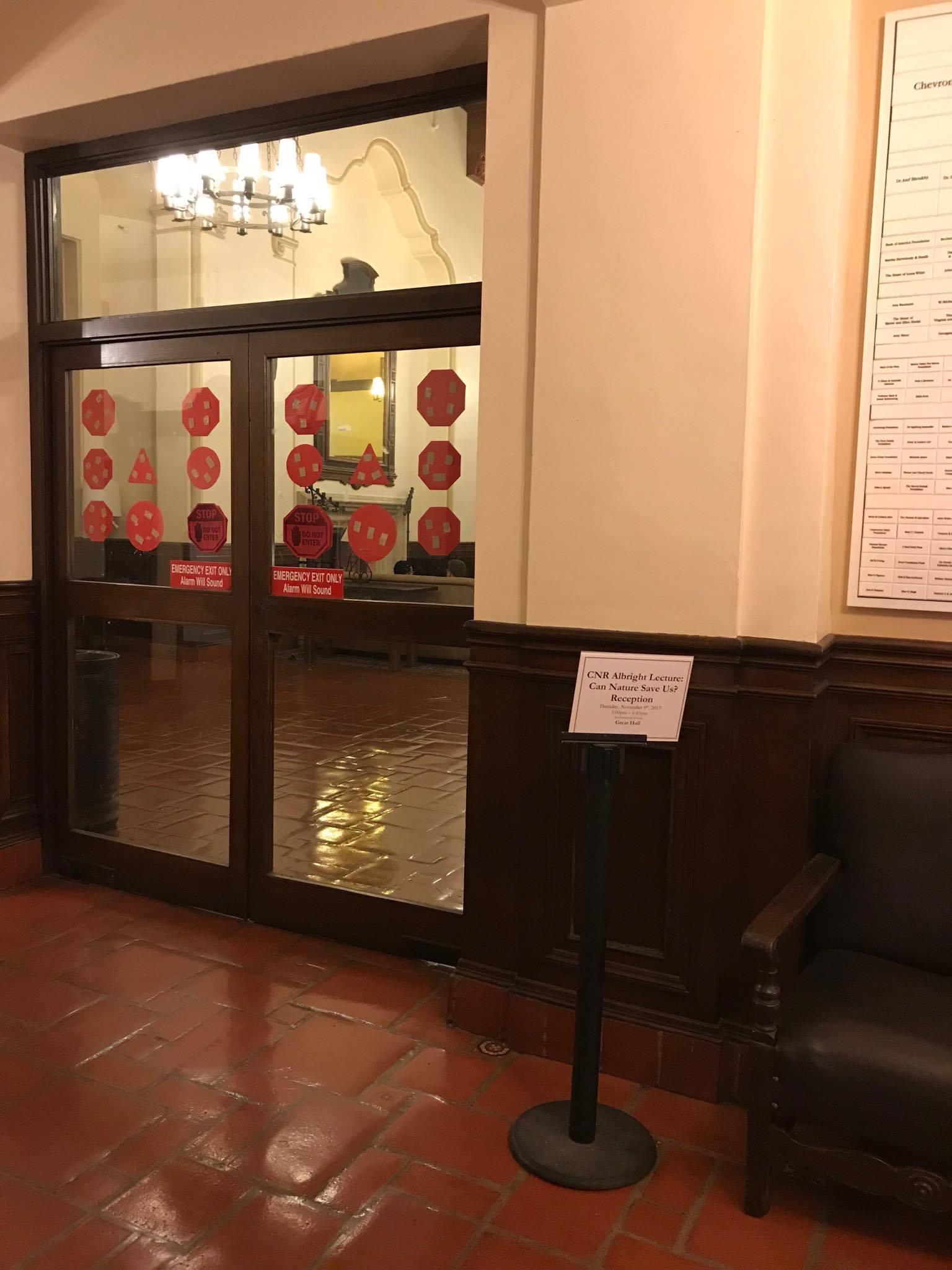
Right Image of ihouse door
In this part we recover the transformation between each pair of images, which are called homographies. We need to have at least 4 pairs of points (p) to be transformed to a different 4 pair of points (p') and solve for a 3x3 matrix of 8 unknowns ([a, b, c], [d , e, f], [g, h, 1]) and a value of 1 (H). We will solve for H with the equation p' = Hp. Set up a system of linear equations Ah = b where h is an 8x1 vector of the unknown values from H ([a, b, c, d, e, f, g, h]), b is a vector of the x, y coordinates from p', and A is a matrix where for each x,y coordinate pair from p corresponds to a rows of the form [x y 1 0 0 0 −xx′ -yx′] and [0 0 0 x y 1 −xy' −yy']. If there are more than 8 equations then use a least square solver otherwise we can solve the normal way.
Since we found the homography from set of points p to set of points p', we can warp images to a different plane. I used the warp function from the skimage transform package to achieve this with the inverse map being our recovered homography. In the images below, you can see that I warped the MLK amazon picture to the TV, the I House door to the left door, and the I House Cafe to the Just Go refridgerator.
Warped MLK Amazon Store
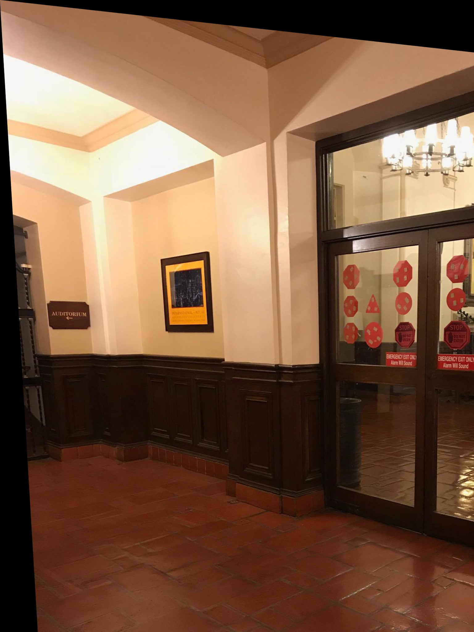
Warped iHouse door
Warped iHouse cafe
Once we have the warped left image as well as the right image. I manually found the seam in which it matched the image perfectly and linearly blended the image together. You can see the results below!
Final MLK Amazon Store
Final Ihouse Cafe
Final Ihouse Door
The coolest technique I learned was how to recover homographies. This allowed us to warp images to a different plane and stitch them to another image of similar plane. It's super useful in creating panoramas and is extremely powerful in other applications!
To demonstrate the auto alignment procedure, I will use the following pictures as seen below...
Left Image of MLK Amazon Store
Right Image of MLK Amazon Store
I used the python starter code in harris.py to detecte Harris Interest Points. Since, harris interest points are measured by their corner response, the higher the response at a point the stronger of a harris corner it is. As you can see below I have displayed the harris corners for my example images.
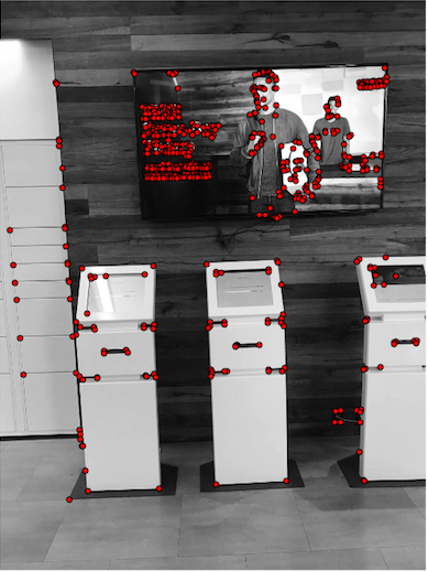
Left Image of MLK Amazon Store
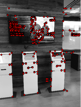
Right Image of MLK Amazon Store
I based my ANMS implementation on the description stated in the paper. We need ANMS as it limits the number of points to consider in the following steps. If we didn't do this, our algorithm would take forever.The basic idea of ANMS is to keep the strong Harris corners which are also well-distributed spatially across the images. I used the formula in the paper to find the minimum supression radius. Below are the refined points using the ANMS algorithm.
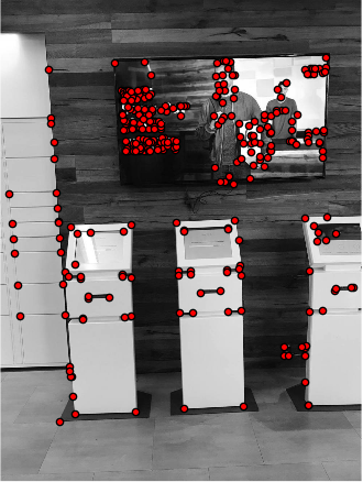
Left Image of MLK Amazon Store
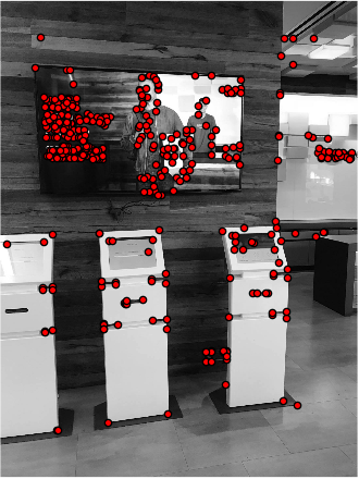
Right Image of MLK Amazon Store
We now need to find a feature descriptor for each of the points chosen by ANMS. This will allow us to develop a point correspondence between our 2 selected images. I followed the paper's instructions to build the feature descriptor described in the MOPS paper. We needed to examine 40x40 patch surrounding for a given Harris interest point. I convolved the patch with a Gaussian and then downsized it to an 8x8 patch. This allows us to be faster when comparing different point similarities. I then subtracted the mean and divided by the standard deviation to adjust for bias and normalization.
Now we need to actually match the points and create the correspondence. I used a SSD metric (used dist2) on the feature descriptors, comparing each feature descriptor in one image to all the other features in the other image. In the paper it talked about the Lowe algorithm. I used this approach to do feature matching. Essentially I found the 1-NN, the SSD error of the first nearest neighbor, or best match, for each feature descriptor, and then 2-NN, the SSD error of the second nearest neighbor or second best match, and then looked at 1-NN/2-NN. After running this algorithm, the points that were left over were essentially the points that had distinct matches.
Now we need to actually match the points and create the correspondence. I used a SSD metric (used dist2) on the feature descriptors, comparing each feature descriptor in one image to all the other features in the other image. In the paper it talked about the Lowe algorithm. I used this approach to do feature matching. Essentially I found the 1-NN, the SSD error of the first nearest neighbor, or best match, for each feature descriptor, and then 2-NN, the SSD error of the second nearest neighbor or second best match, and then looked at 1-NN/2-NN. After running this algorithm, the points that were left over were essentially the points that had distinct matches.
Great, we have our correspondence points! However, there are a couple of things that we have to do before finishing up the autostitching process. We need to compute the homography between the images. Since, there might be outlier points, we need to filter them down and find the best points. I used the RANSAC algorithm which takes 4 random points in one image and uses them to compute a homography using their correspondences in the other image. For every point in the original image, I transformed it using the homography and calculated the distance of the transformed point to the actual point correspondence. I looked at |p′i−Hpi||pi′−Hpi| and if this distance is less than a certain threshold, then I said that the point pipi agreed with the homography HH. After doing this multiple times, I chose the optimal homography which had the most points agreeing with it.
Below are my results! Some images came out better than the manual stitching, but other images were worse. The best explanation I can give, is perhaps there weren't that many good objects of focus in backgrounds that were pretty uniform such as the amazon store and the ihouse cafe.
Auto Stitch MLK Amazon Store
Manual Stitch MLK Amazon Store
Auto Stitch Ihouse Cafe
Manual Stitch Ihouse Cafe
Auto Stitch Ihouse door
Manual Stitch Ihouse door
I learned that autostitching is a very powerful algorithm and that we can distill down complexities into very tangible mathematic concepts.