CS194-26 Project 6: Image Warping and Mosaicing A&B

YiDing Jiang

Overview

In thie project, I will blend and stitch multiple images together to create an "image mosaic" or a panorama. To achieve this, I first choose one image, usually the center one as the anchor and then pick corresponding feature points on all the images. These feature points are in turn used compute homographies that encodes the perspective transformation that warp the neighboring images onto the center image. After obtaining the homographies, inverse warping is used to transform the neighboring images into property location and geometries so they can be blend together. For blending, I use a linear blending technique over the regions of overlap which removes the edge artifact reasonably well.

1. Compute Homography

Given 4 or more pairs of corresponding features, we can compute a perspective transform of 8 parameters that can transform one into a geometry that matches the other. In principle, 4 points provide 8 equations to solve the homography, but in practice because of labeling error and imperfection of the pictures taken, using more than 4 points and least square linear regression would give much better results than 4 points alone, assuming there is no systematic bias in the noise. Formally, for all pairs of points in $$(\begin{bmatrix} x_i \\ y_i \end{bmatrix}, \begin{bmatrix} x_i' \\ y_i' \end{bmatrix} )$$ given, we seek $$H \in \mathbb{R}^{3,3}$$ that minimizes $$\sum_i ||H\begin{bmatrix} x_i \\ y_i \\1\end{bmatrix}-\begin{bmatrix} wx_i' \\wy_i'\\w \end{bmatrix}||_2^2$$ in homogeneous coordinate.

Suppose $$H = \begin{bmatrix} a & b&c \\ d&e&f \\ g&h&1\end{bmatrix}$$ , $$H\begin{bmatrix} x \\ y \\1\end{bmatrix} = \begin{bmatrix} wx' \\ wy' \\w\end{bmatrix} = \begin{bmatrix} ax+by+c \\ dx+ey+f \\gx+hy+1\end{bmatrix}$$ .

Since $$w=gx+hy+1$$ , we can do a further substitution $$\begin{bmatrix} ax+by+c \\ dx+ey+f \\gx+hy+1\end{bmatrix}= \begin{bmatrix} (gx+hy+1)x' \\ (gx+hy+1)y' \\gx+hy+1\end{bmatrix}$$ .

Rearranging the terms we have $$\begin{bmatrix} ax+by+c -gxx'-hyx' \\ dx+ey+f -gxy'-hyy'\\gx+hy+1\end{bmatrix}= \begin{bmatrix} x' \\ y' \\gx+hy+1\end{bmatrix}$$

The above equation can be equivalently expressed as $$\begin{bmatrix} x & y & 1 &0&0&0&-xx'&-yx' \\ 0 & 0 & 0 &x&y&1&-xy'&-yy' \end{bmatrix} \begin{bmatrix}a\\b\\c\\d\\e\\f\\g\\h\end{bmatrix} = \begin{bmatrix} x' \\ y' \end{bmatrix}$$ .

We can solve for $$a,b, \dots, h$$ by setting up matrix $$A$$ and target $$b$$ with all $$(x,y),(x',y')$$ pairs and solving it with linear regression.

2. Warp the Images

The warp is done through inverse warpping and bilinear interpolation to avoid artifacts and aliasing. One special thing that needs to be done for image mosaic is that I had to estimate the resulting image, create a blank canvas of appropriate size and put the center image at the center of the canvas so everything can be done on the canvas. Also note that applying the homography makes $$w\ne1$$ so I normalize the transformed homogeneous coordinate by corresponding $$w$$ to project them back onto the image plane.

3. Image Rectification

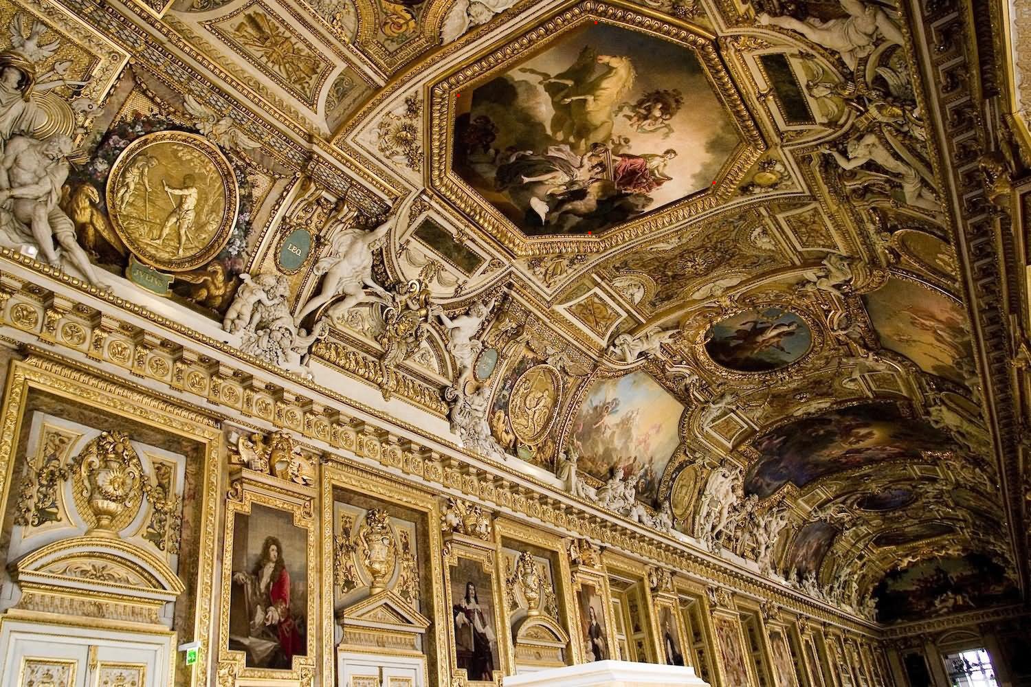
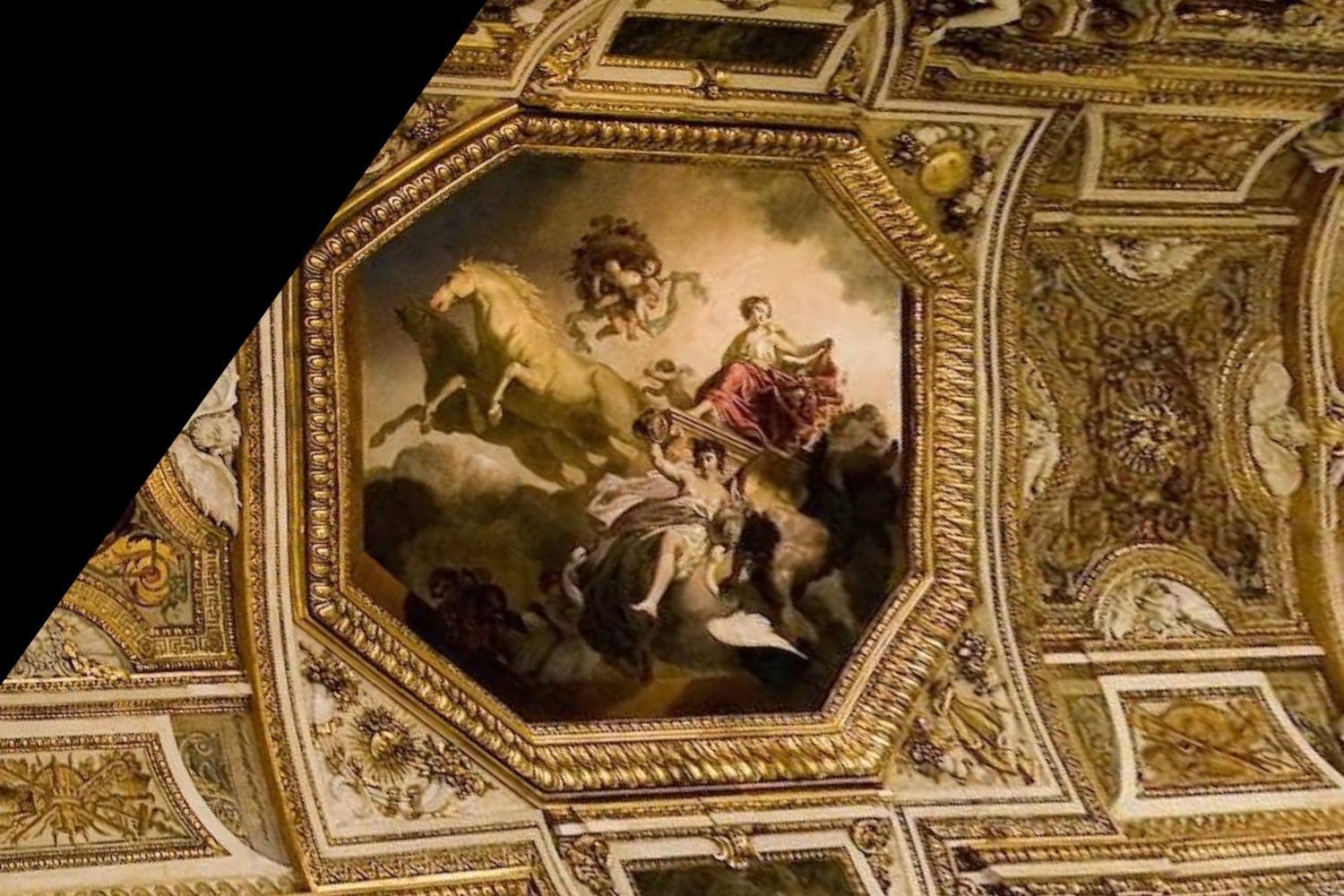
With tomography computed on 4 pair of points, I could recover the exact transformation that transforms an image at some angle into a nice rectangle. If the original image is assumed planar, this can be used to recover the front view of a rectangular plane.

Original Image	Recified Image

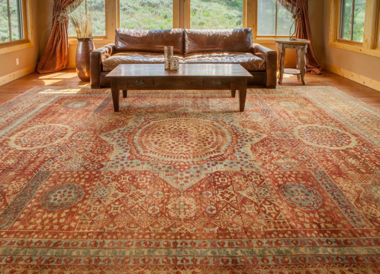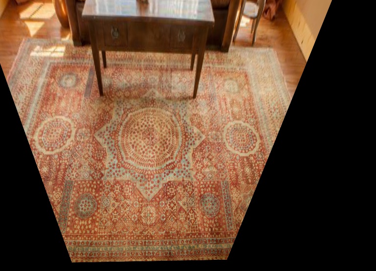Through tomography, I am able to recover the front view of the painting on the ceiling of Louvre. (Four points are labeled red in the left image if you look hard enough...)

4. Image Mosaic

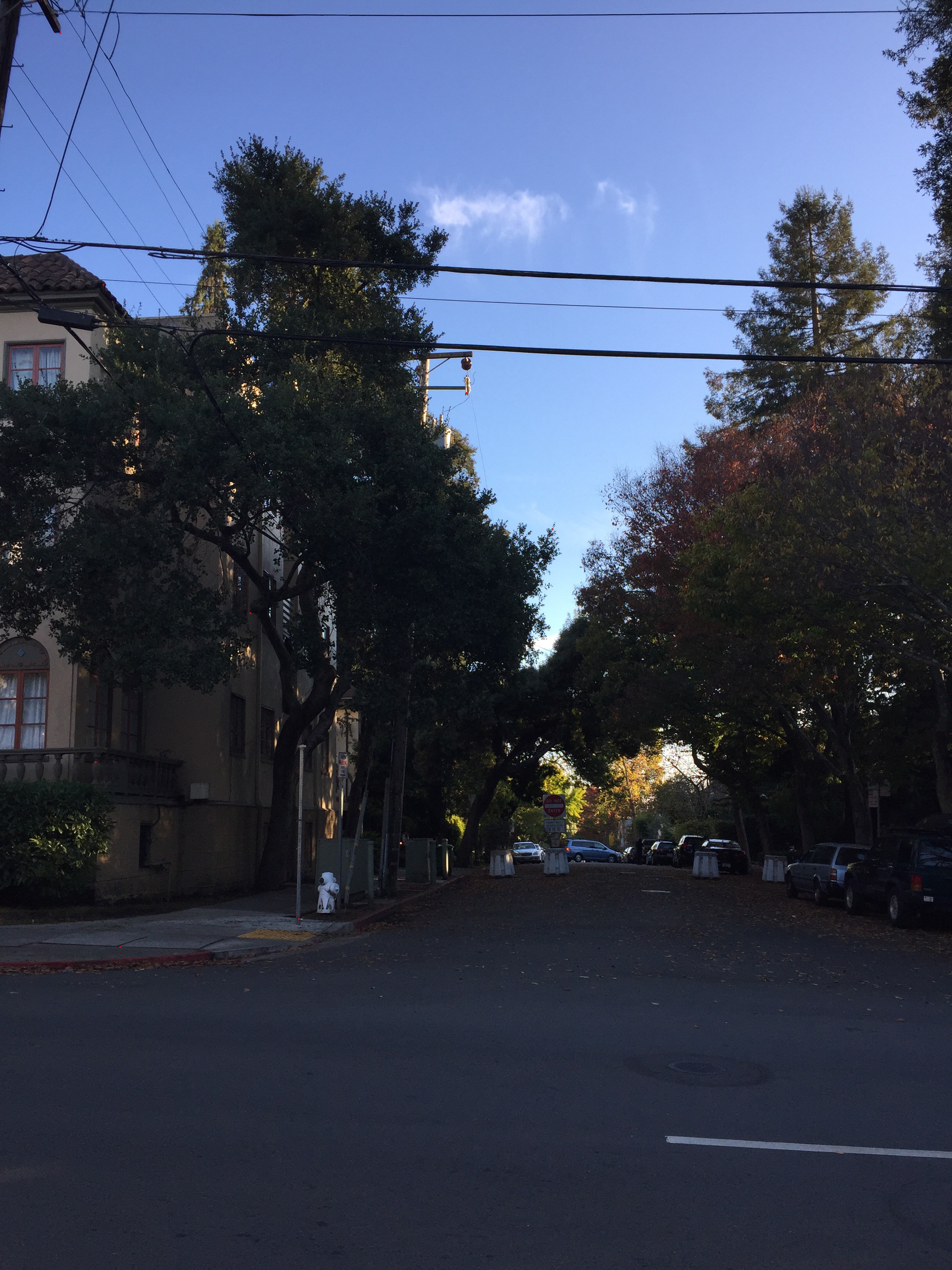
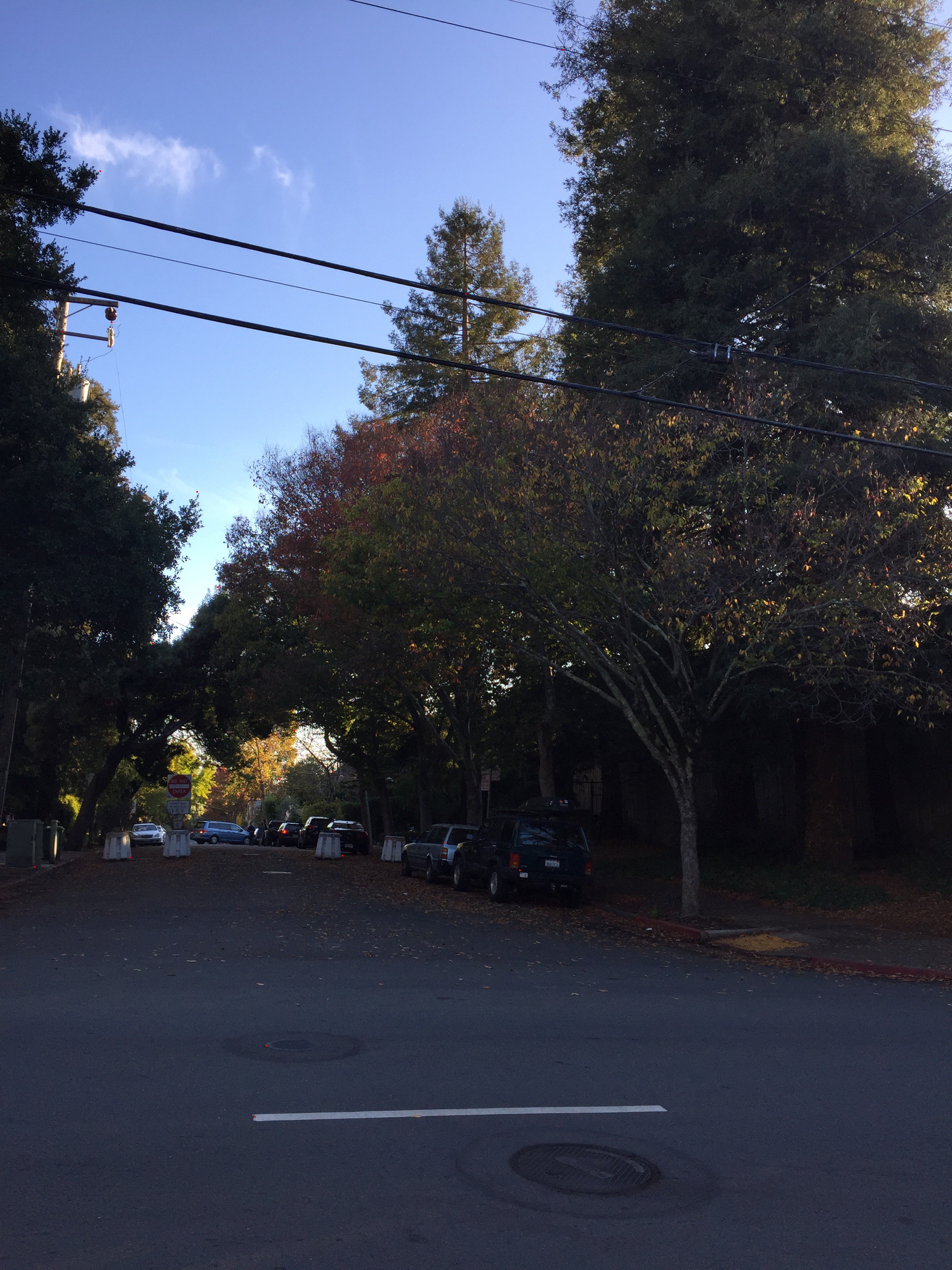
Given two or more images, I first choose an image as the anchor and warp the rest to align the feature points.

Left Image	Right Image

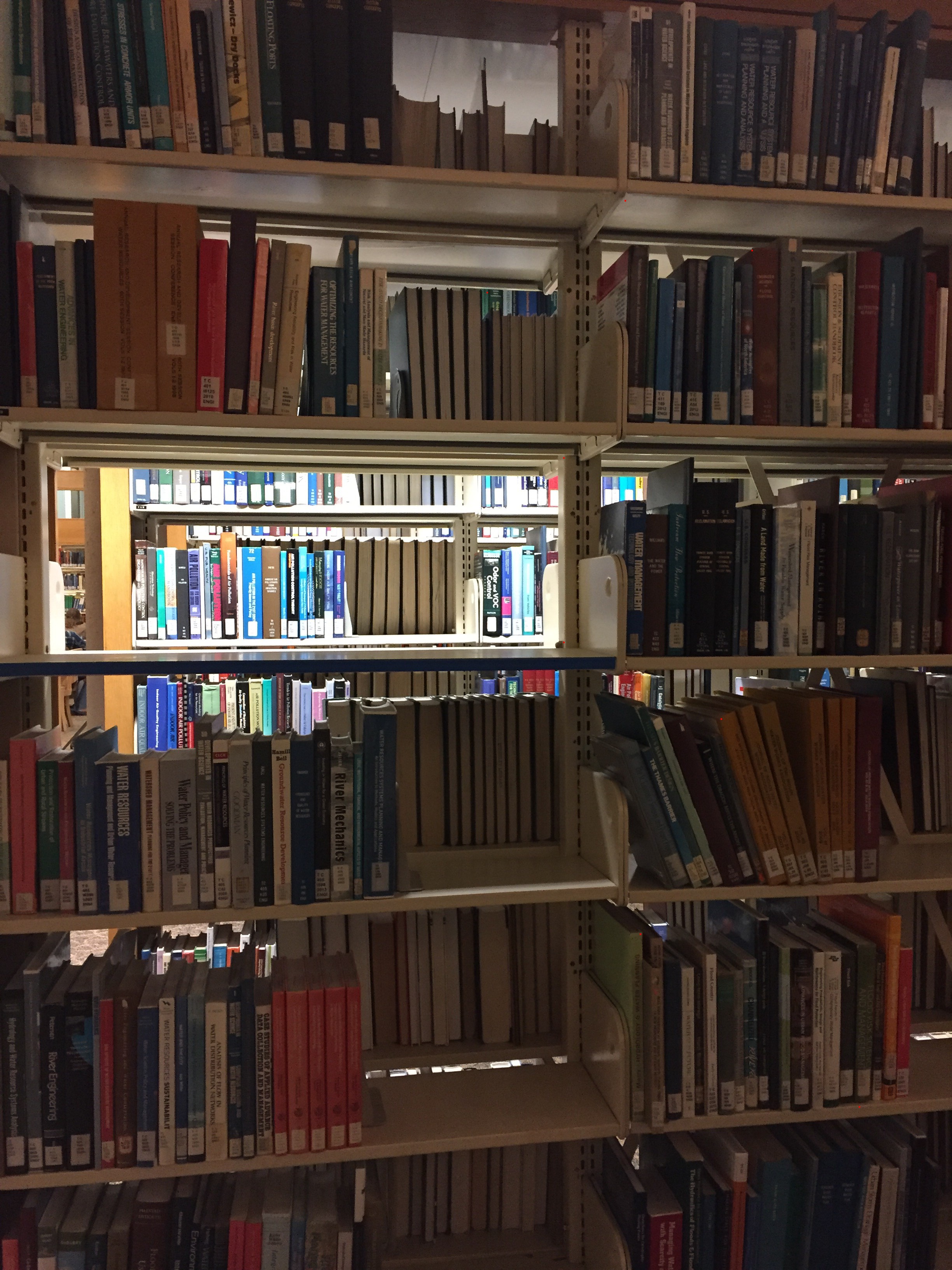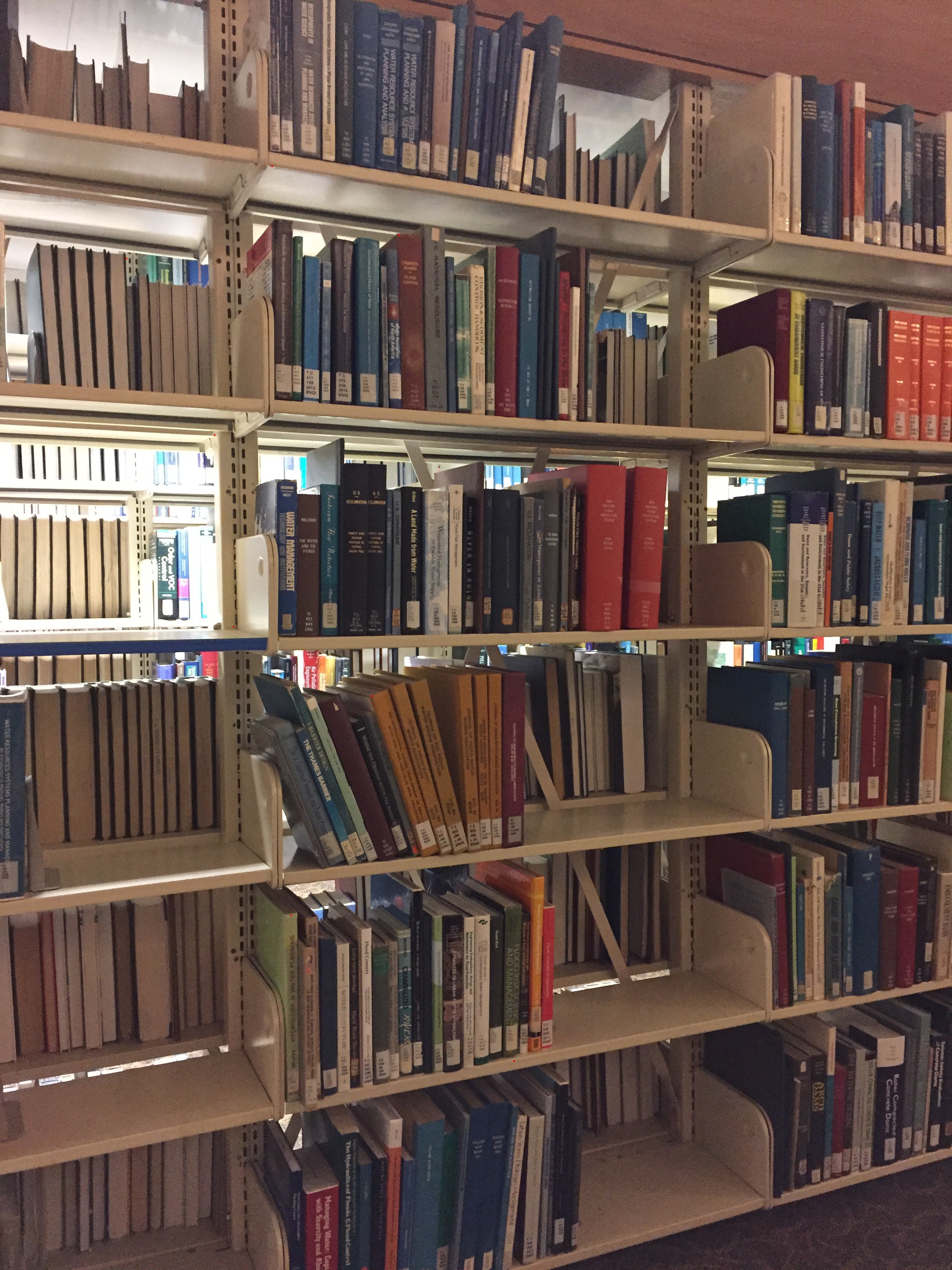Kresge Mosaic (Linear blend)

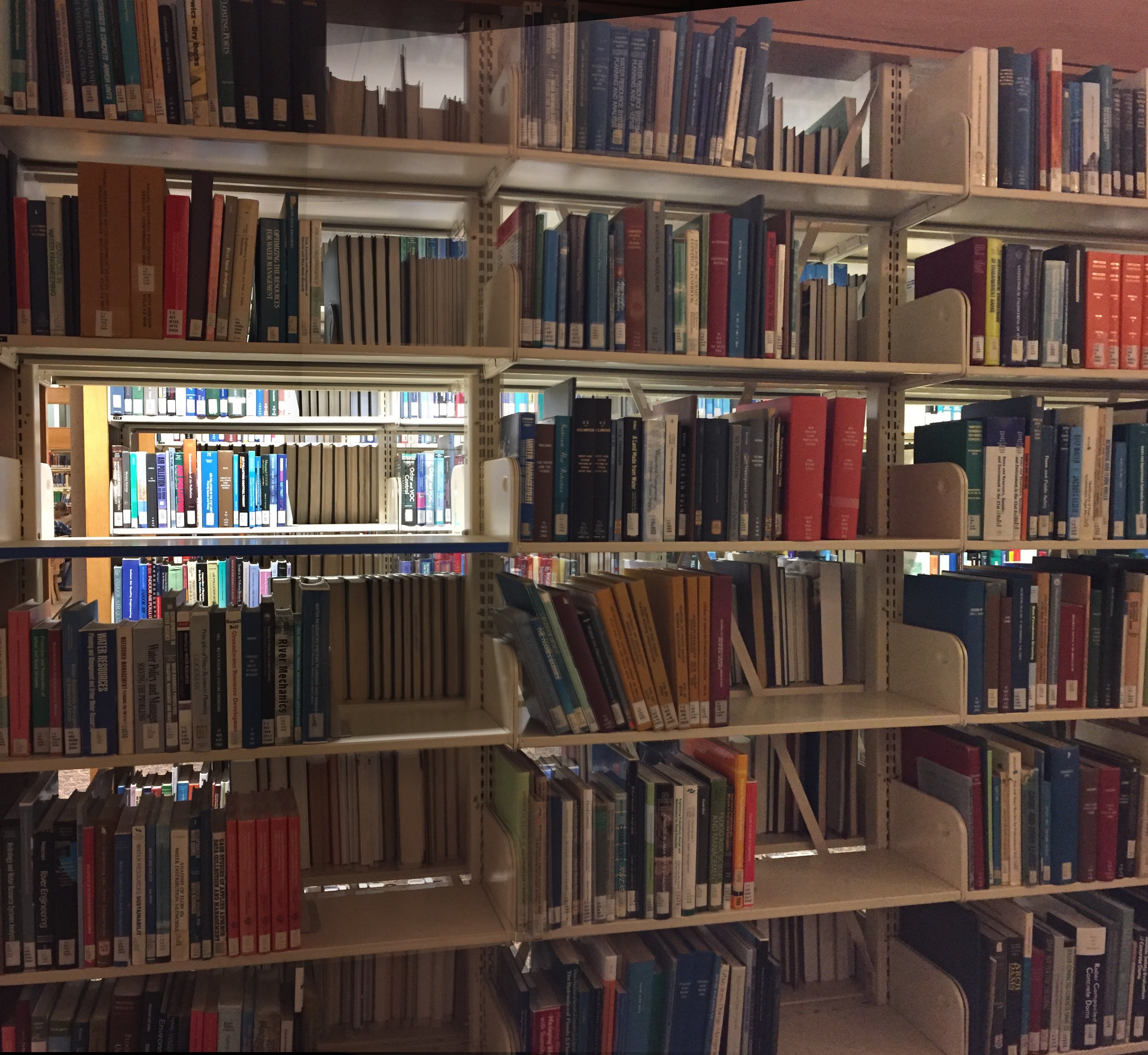Note that even though the two images have very different lighting, the linear blend worked quite well except at the bottom and top where the geometries of the two images mismatch.

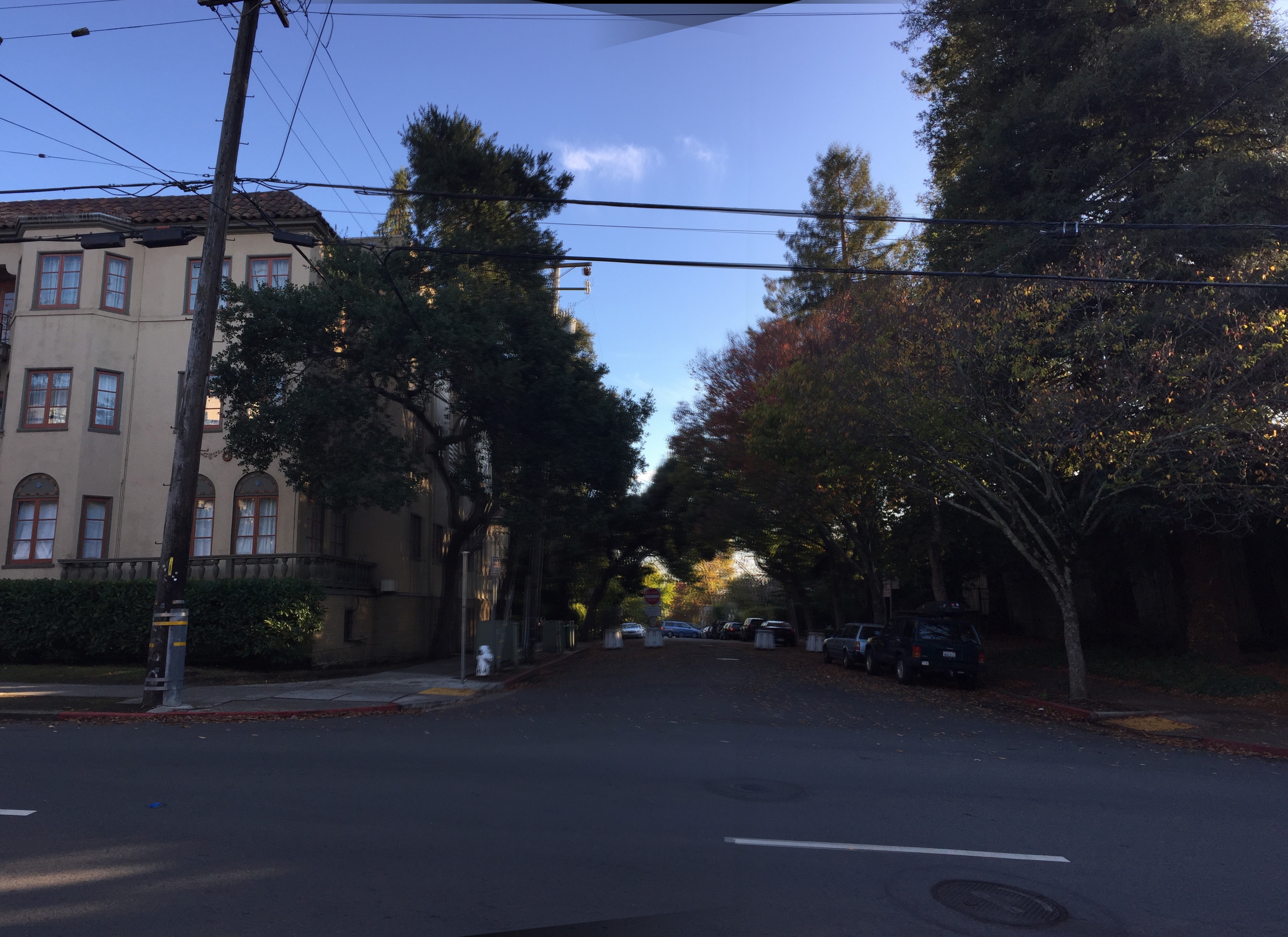
For 3 images blend, I use the approach of growing the mosaic one image by one image — adding one to the mosaic of previous 2 by doing 2 mosaics.

Left	Middle	Right

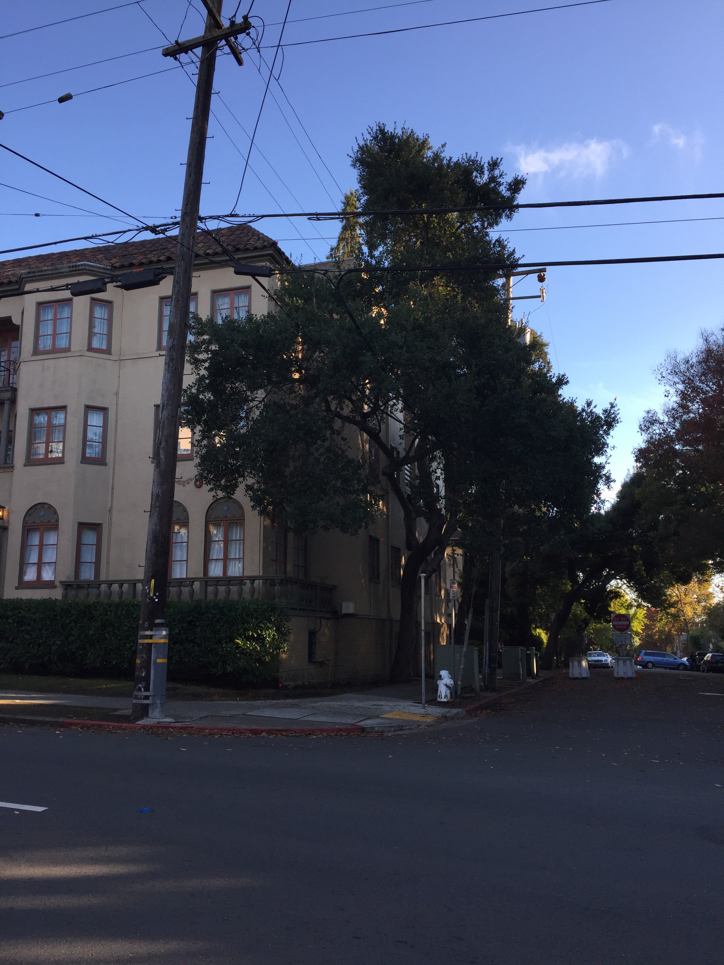2 Mosaics Together (Linear blend)

Notice that linear blending works really well in terms of blending colors and removing edge artifacts; however, when there is a lot of predominant high frequency components such as the leaves, naive linear interpolation will result in small ghosting because the feature points are hand labelled and contain non-trivial error. This problem is solved in part B by using automatic feature detection.

Example blending masks:

Left Mask	Right Mask

Dark area are 0 and white areas are 1. This is multiplied to the left image and right image before adding them together. This is the equivalent of linear interpolation between pixel values of two images.

Part B:

5. Harris Corners and Adaptive Non-Maximal Suppression

The work above involves painful hand picking feature points on the images and these handpicked points are usually not accurate on the pixel level as humans are not perfect. This process can be automated through algorithms which are much more reliable and accurate than humans.

Using the provided Harris corner detector, we can extract all potential corners in the images that can be paired together. However, the algorithm naively returns many candidate corners which cover the entire image and is not very informative. Instead, I only pick the corners with top ~120000 corner responses.

Thresholded Harris corner detection	ANMS

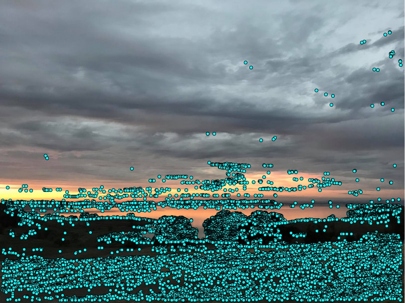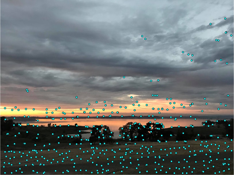As you can see, the results are still not great as there are points everywhere in the image. We can improve the corner detection by using ANMS where we found $$r_i = \min_{ \forall j\ne i} ||x_i - x_j||_2$$ such that $$f(x_i) \leq 0.9 f(x_j)$$ for every corner $$x_i$$ ( $$f(\cdot)$$ is the strength of the corner). This optimization finds the nearest corner where corner $$i$$ has a weaker corner response than and 0.9 is the robust coefficient. We can pick the corners with the top 500 suppression radii to ensure that the points are well spread out on the image.

6. Feature Descriptor Extraction

With more evenly spread out corners detected, we can extract 40 pixel by 40 pixel feature patches center at each corners in both images and try to establish correspondence. We first down sample the patches to 8 pixel by 8 pixel through Gaussian pyramid and then standardize the patches by center them and divide by standard deviation of each 8x8 feature descriptor.

Example feature descriptor

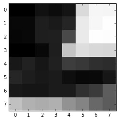7. Feature Matching

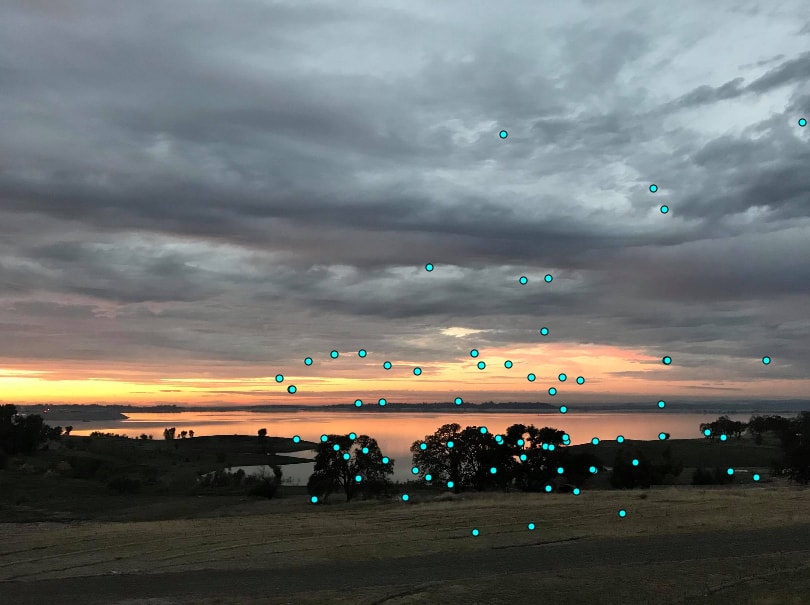
For the feature descriptors of 2 images being stitched, we can run dist2 to find the top 2 nearest neighbors of each feature descriptor. Then we use $$\frac{e(1-NN)}{e(2-NN)}$$ as similarity metric where $$e(\cdot)$$ is the $$l_2$$ difference between the descriptor and one of its nearest neighbor. The idea follows from the observation that mismatches are all mismatched similarly while correct matches are unique. Setting the cutoff ratio to be 0.5, we have matched corner pairs in 2 images:

Left	Right

Note that even though many points are the correctly matched, there are a few outliers that are not matched correctly.

8. RANSAC

We can eliminate the outliers by running the RANSAC algorithm. We first pick 4 corner pairs and compute homography $H$ using the points. Then we compute inliers on all match pairs by finding the pairs where $$|| Hp_i^{(1)} - p_i^{(2)} || _ 2 \leq \epsilon$$ where $$\epsilon$$ is a picked threshold and $$p_i^{(k)}$$ is the $$i^{th}$$ point in image $$k$$ . We use $$\epsilon = 10$$ and repeat the RANSAC algorithm for 10000 iterations, keeping the largest set of inliers.

Then we use all the inliers in the largest set of inliers to compute a robust homography which can be used to stitch the images together.

Left (RANSAC)	Right (RANSAC)

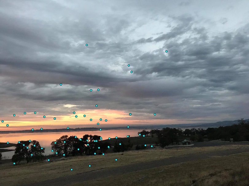Lake Mosaic

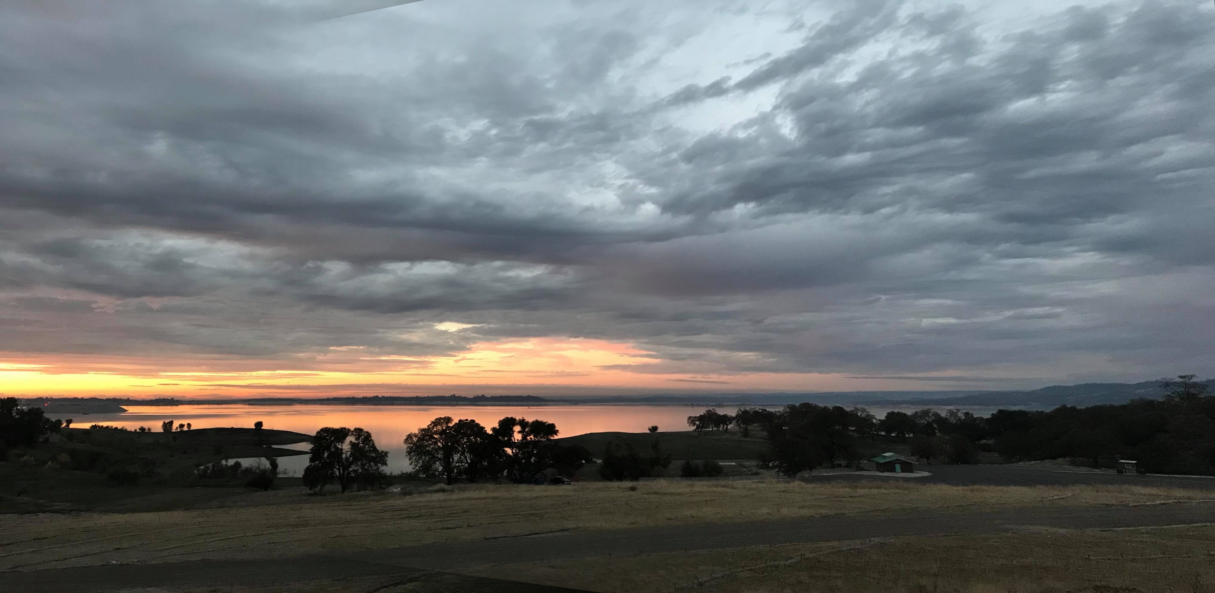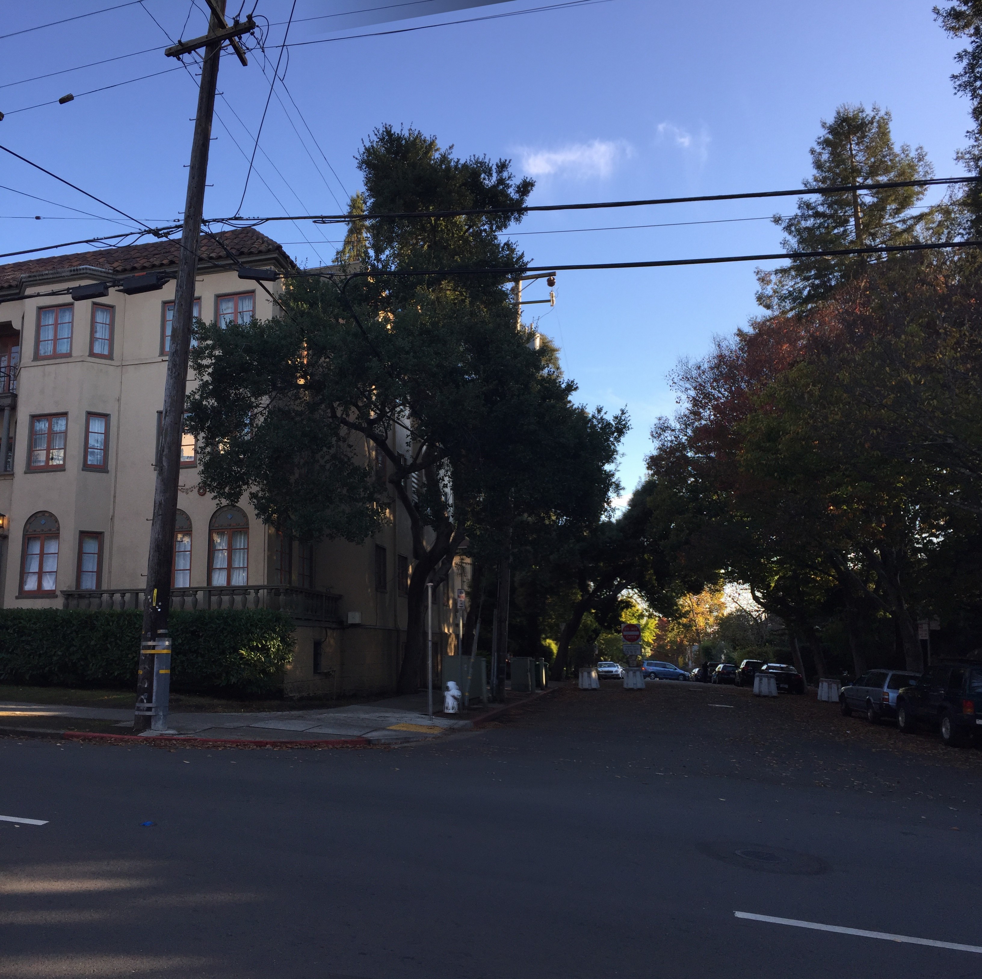
Somewhere in California

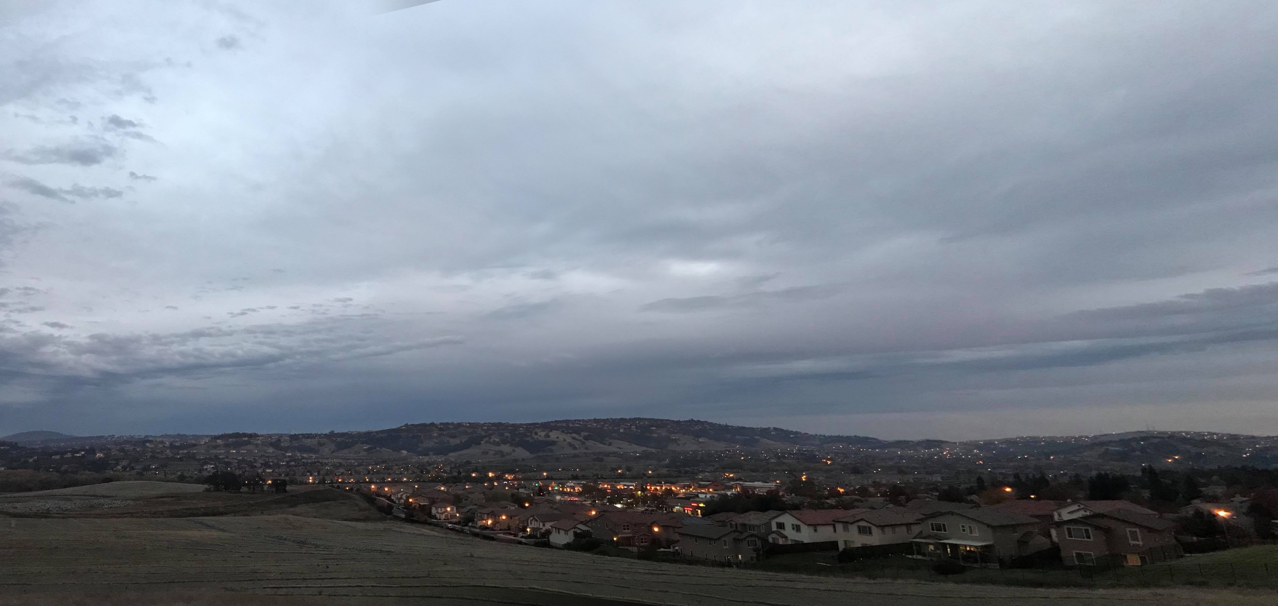Left	Right

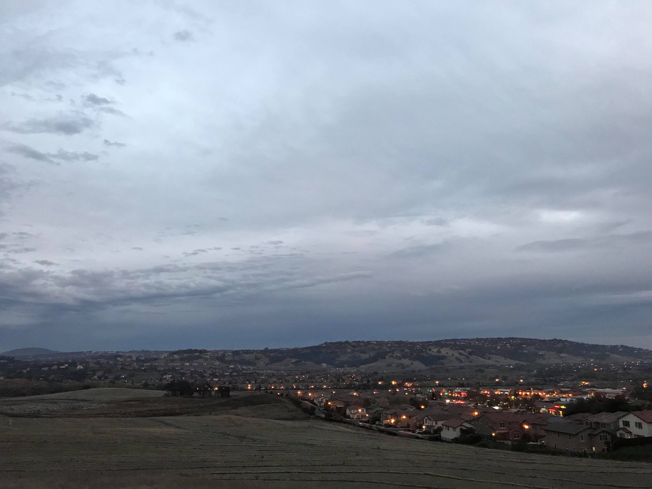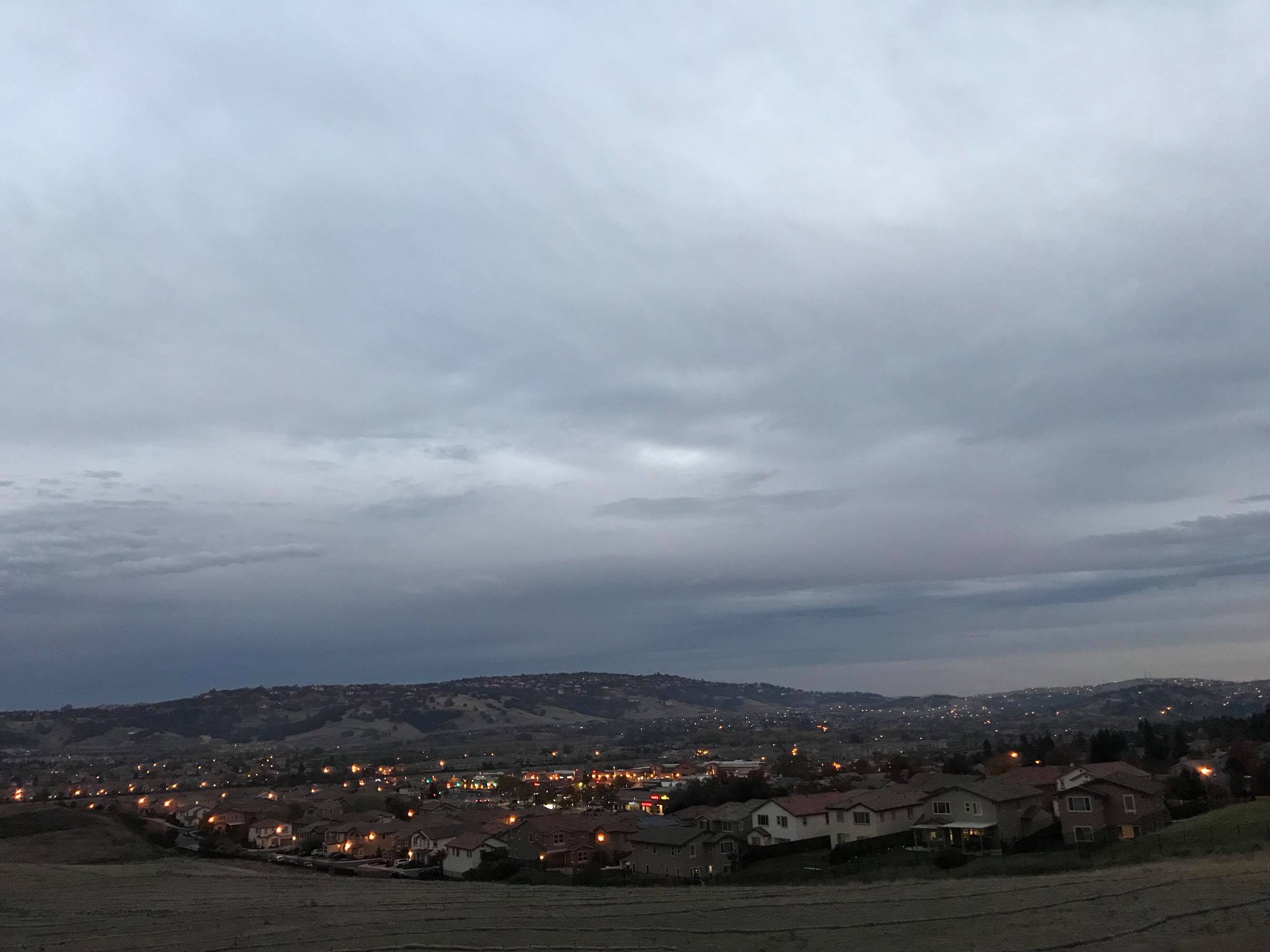For comparison, I ran the algorithm on previous hand labeled data. As you can see the ghosting and misalignment errors that are present in the hand-labelled mosaic are greatly reduced.

Robust Dwight (left and middle)	Hand labeled Dwight (Look at the shadow in left part)

Bells And Whistles

Graffiti

We can use homography to draw graffiti on planar surfaces of photos. We can first threshold the background of the graffiti to make its background black. Then we create an appropriate mask for the graffiti with which we can warp and use it to set target area of the image to be black. Then we can warp the graffiti onto the target image.

Logo	Target

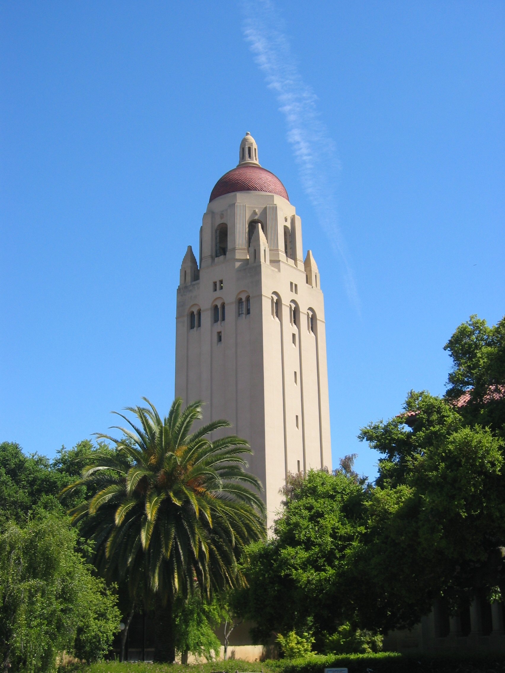How do you not have 4.0 if you can't even step on the seal

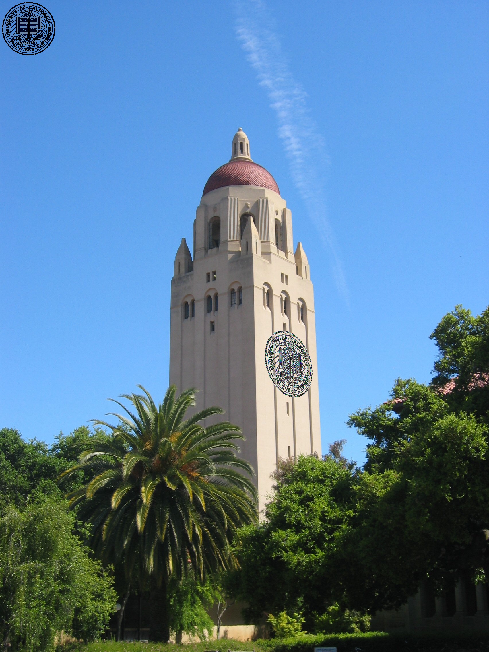Final Thoughts

A very fun project but hand labeling and stitching images together are pretty time consuming. I would like to thank Allan Zhou for sending me nice photos over his break :)