CS 194-26 Project 6

Image Warping and Mosaicing with Feature Matching for Autostiching

By Karina Goot, cs194-aeb

Part 1

Part 2

Introduction

In this project, I worked on creating image mosaics by registering, projective warping, resampling, and compositing images together. This process included a couple of steps all of which are outlined in detail below including capturing and digitizing the images, recovering homographies, warping images together, and finally blending the images into a single mosaic.

Digitizing Images

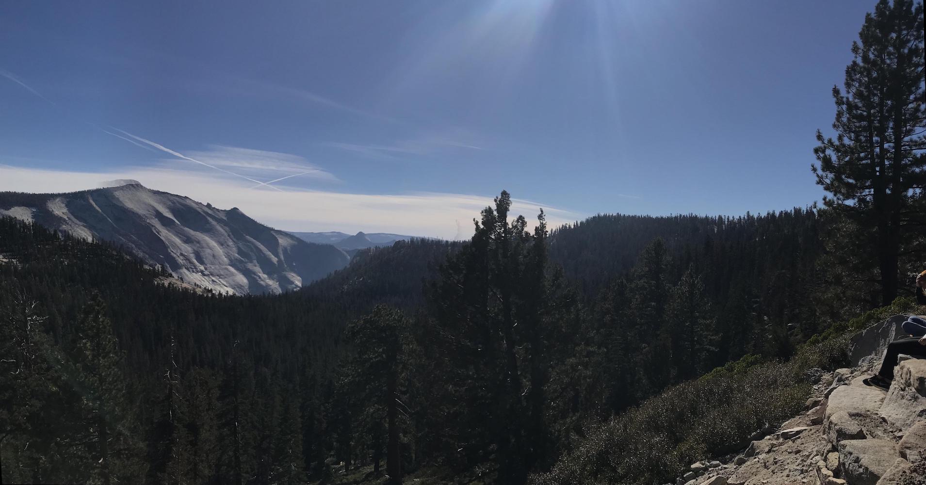
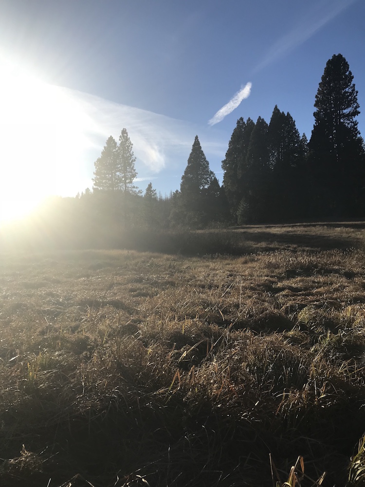
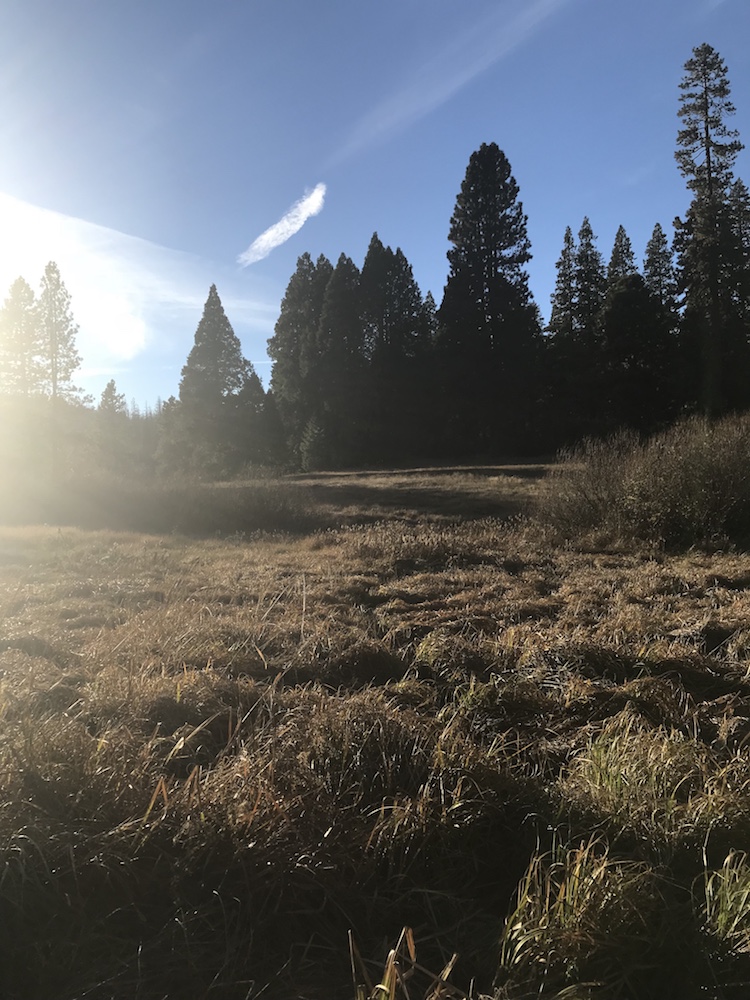
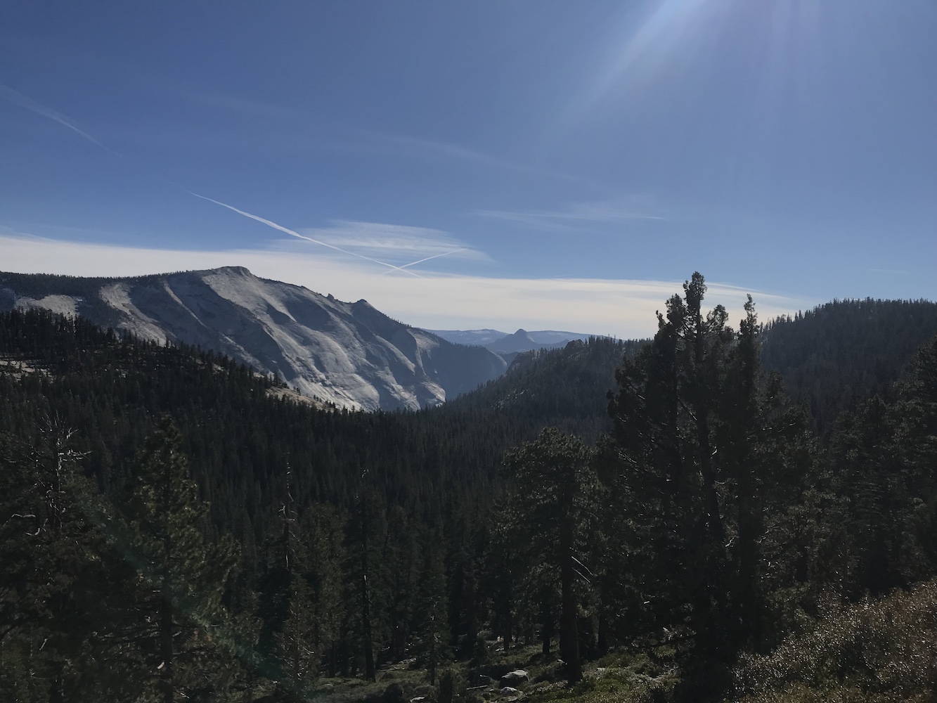
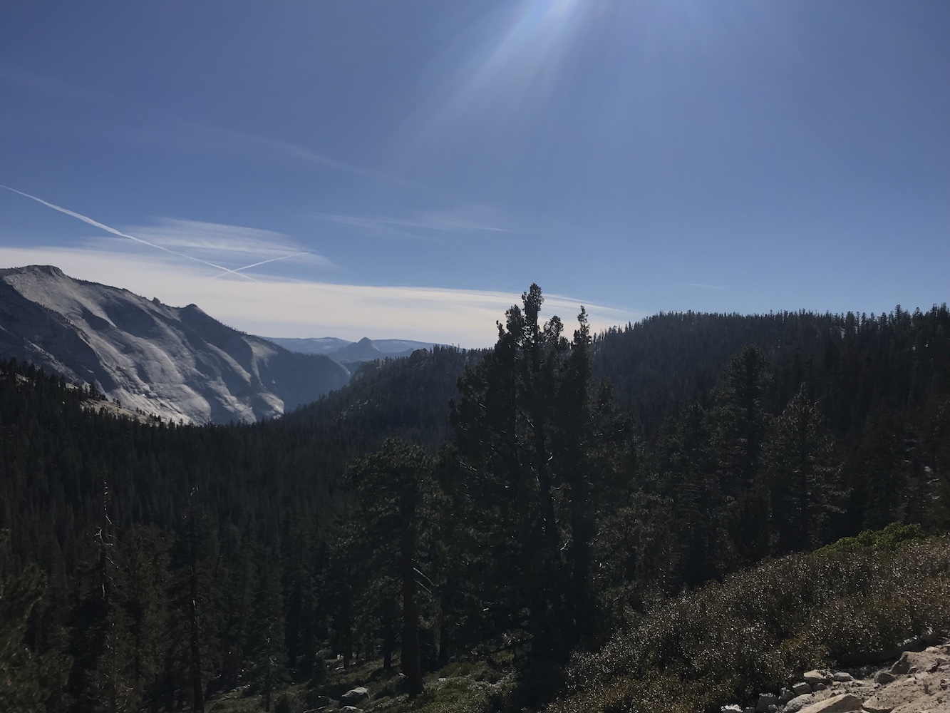
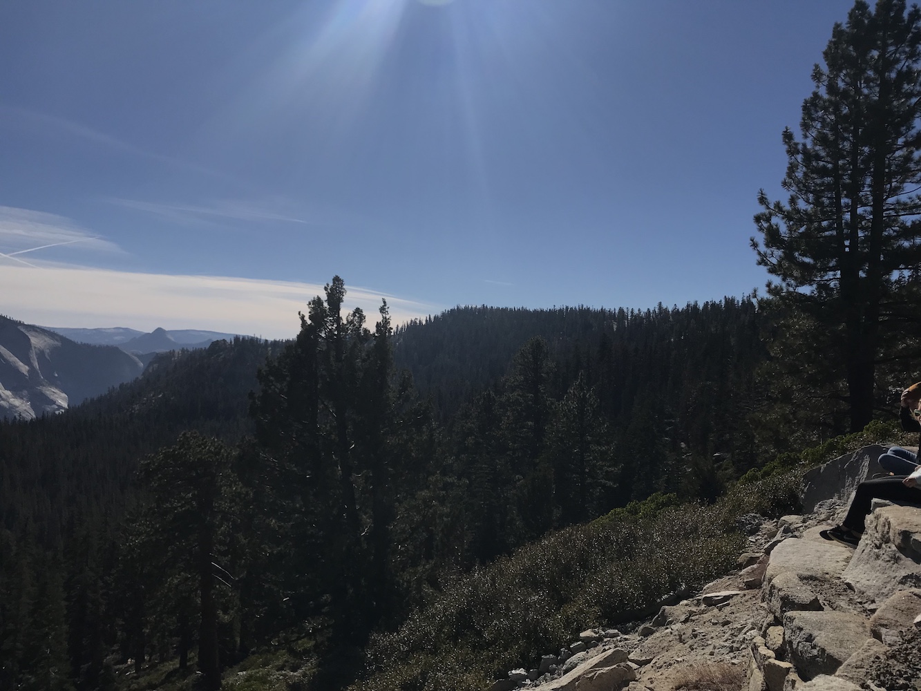
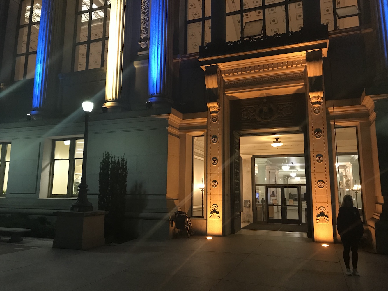
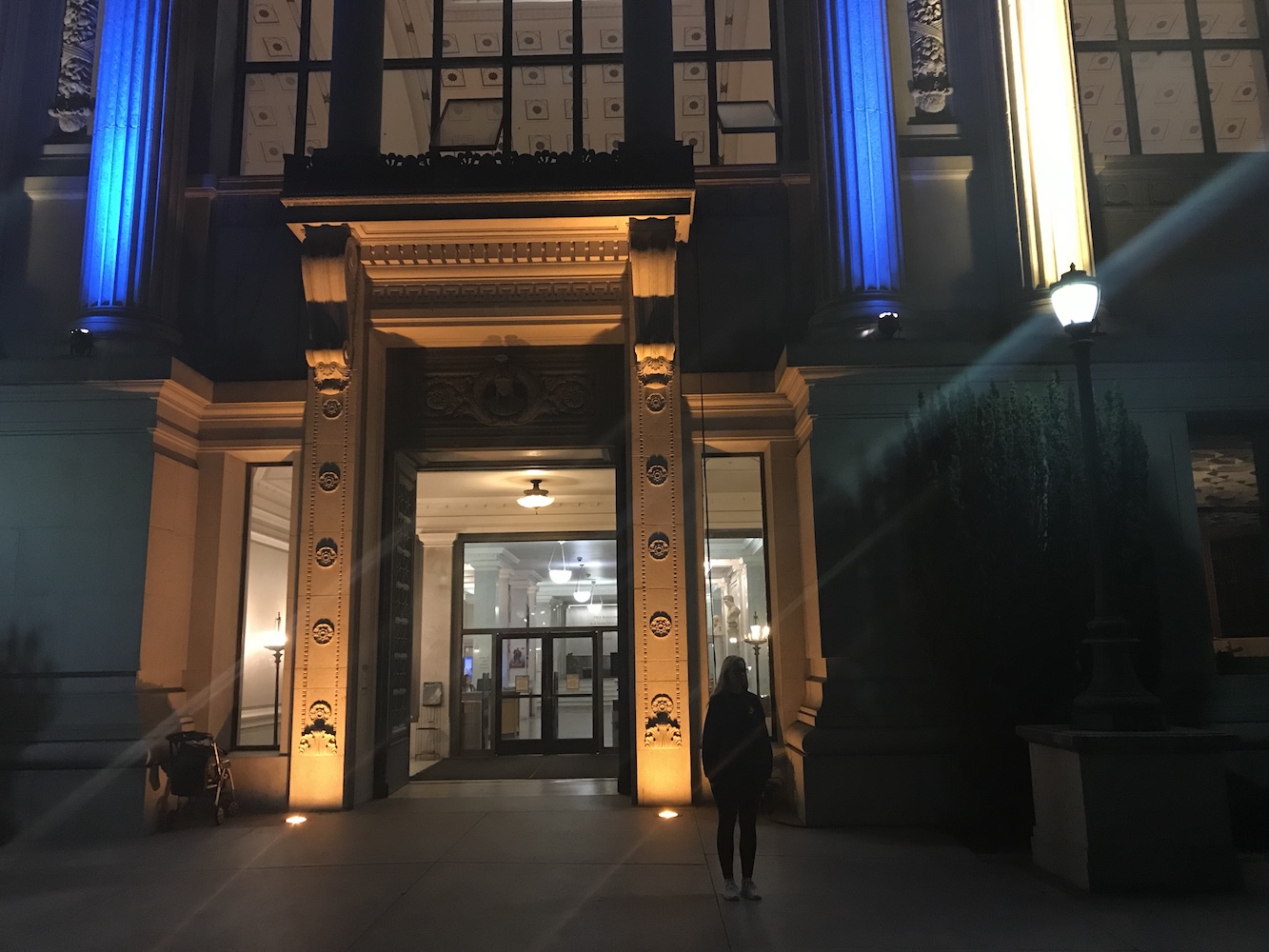
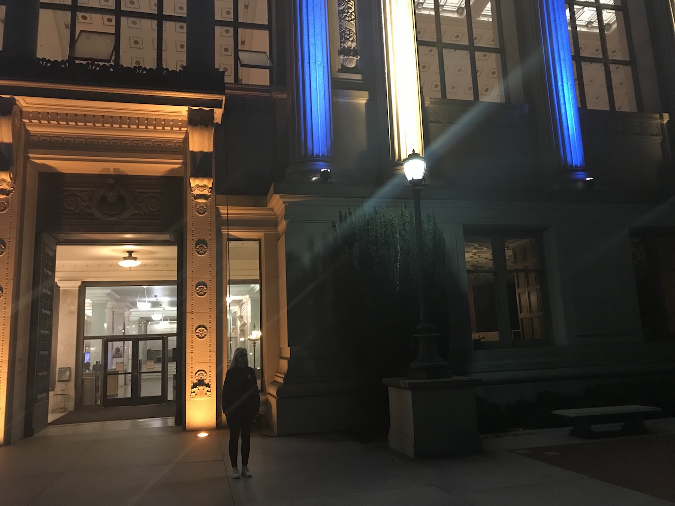
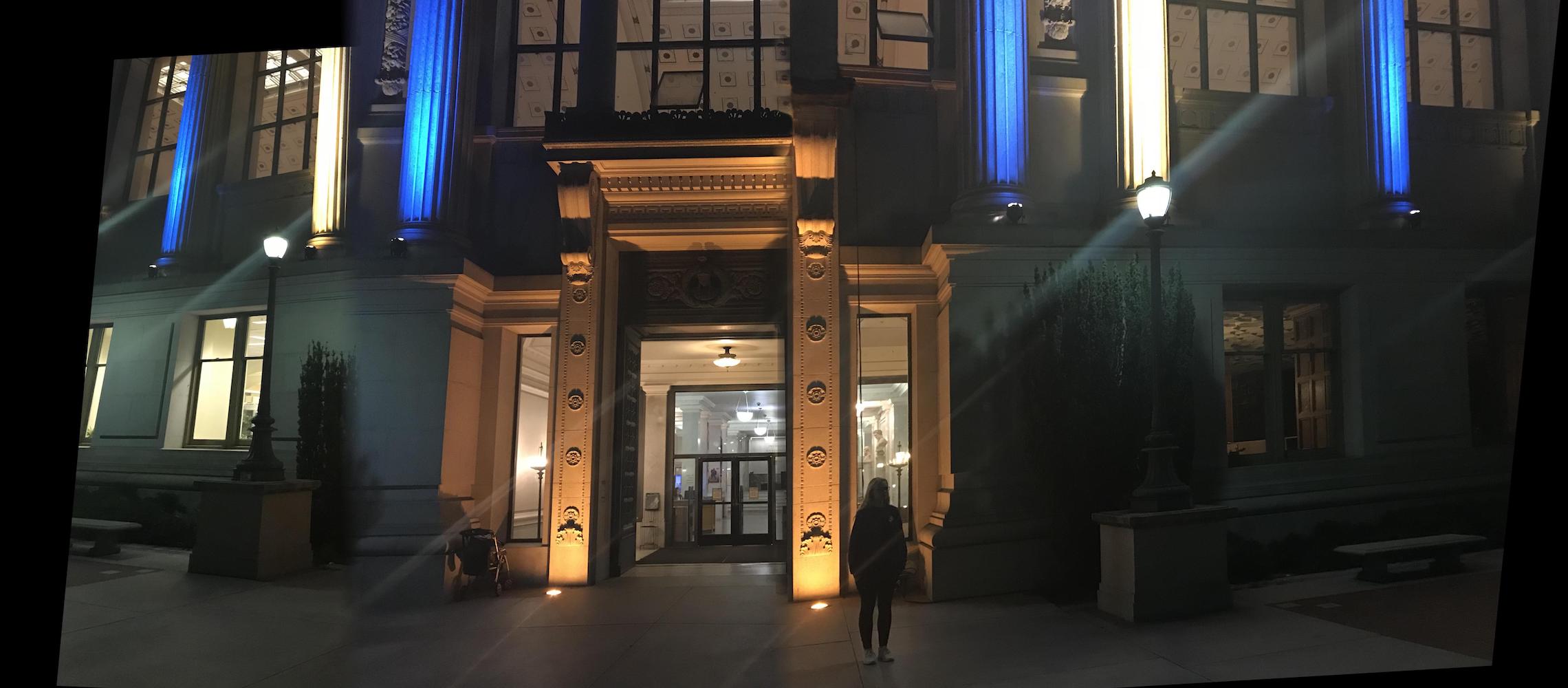
The first part of this project was to capture images. When taking these photos, one of the key considerations was to keep the center of projection identical for sequences of images. I had the opportunity to Hike in Yosemite and decided to take advantage of that and capture series of images for this project. I did not have a digital camera with me while on the trip, the the images I captured at Yosemite were taken on an iPhone7 camera. I did my best to remain still and maintain the camera position as a took photos facing different parts of the scene. I then also decide to try and capture some images during nighttime to see if the effects of the mosaic vary with different lighting conditions, so I captured some images of my roommate on campus at night.

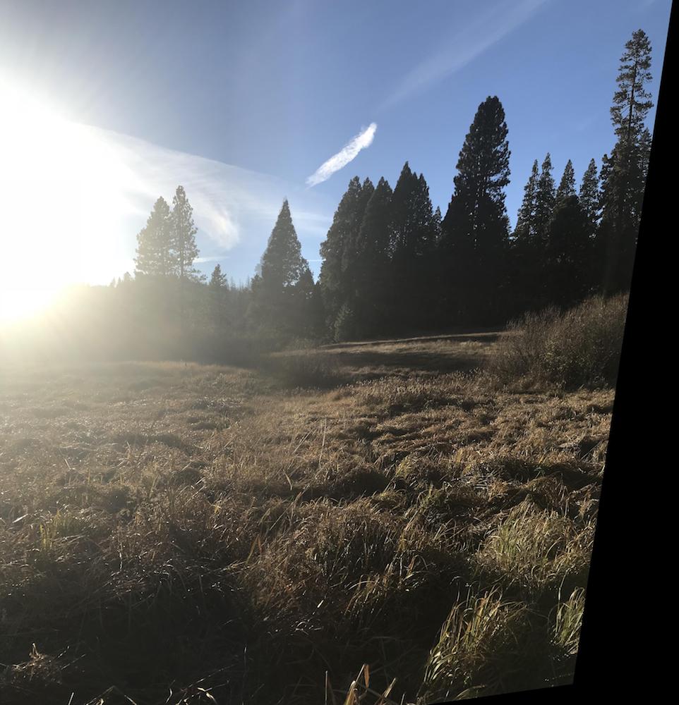
Yellow Meadows

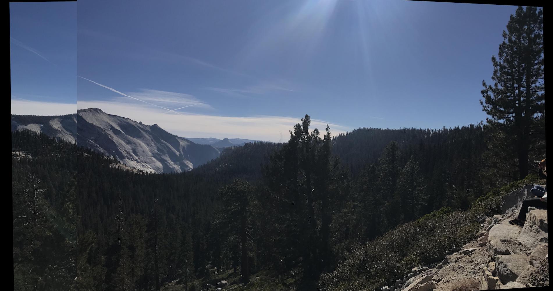
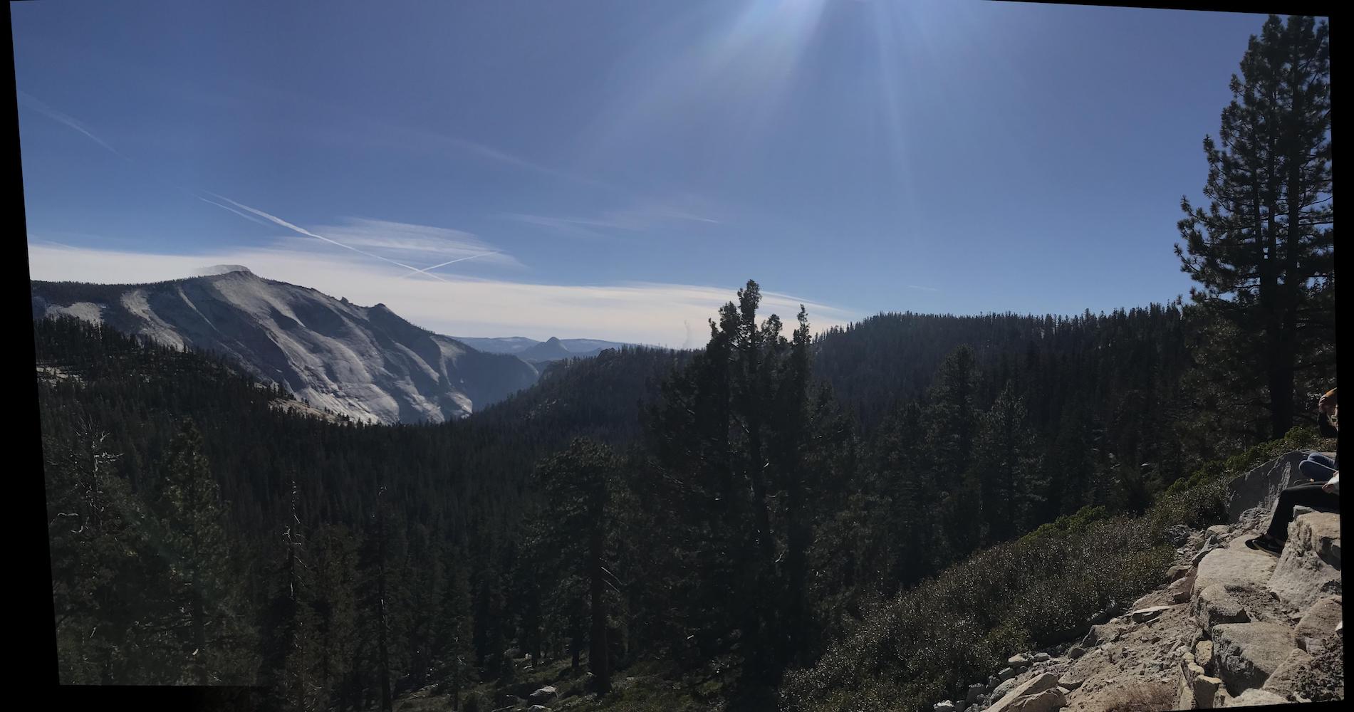
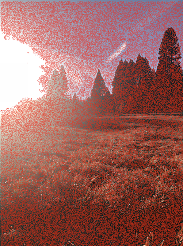
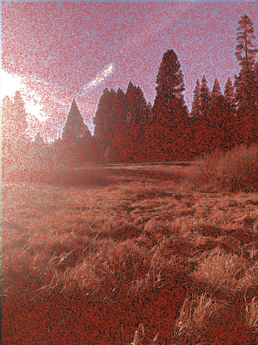
Yosemite Forrest

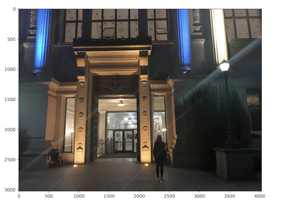
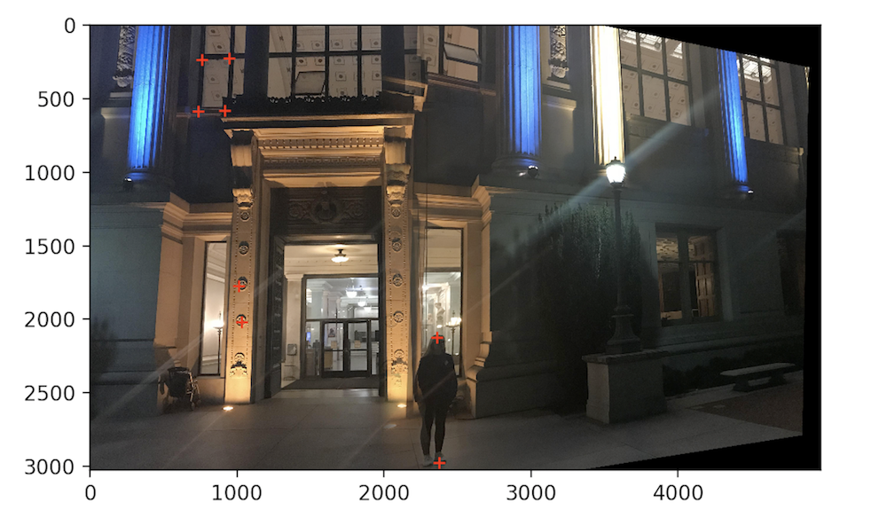
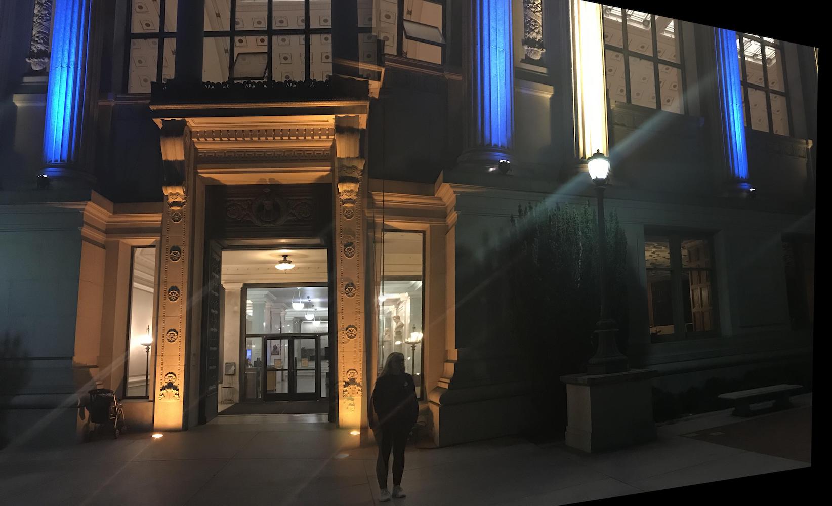
Blue and Gold Lights

Finding Homographies

Now that I had my images captured, I turned to creating projective transformations between the images. These transformations are called homographies and they have 8 degrees of freedom which allow us to transform one image into the plane of another image. In order to solve the homographies, I set up a function,

p' = pH Where H is the homography matrix that holds for this setup:

In order to achieve this, I over-defined pairs of correspondence points between my images and used a least squares solver to find the 8 unknown variables by setting up a system where for each point I added two rows to A and b to then solve for h.

Now I was ready to warp my images!

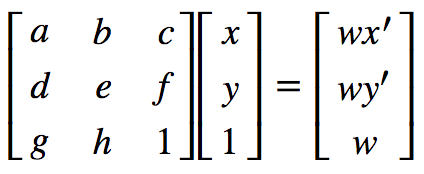
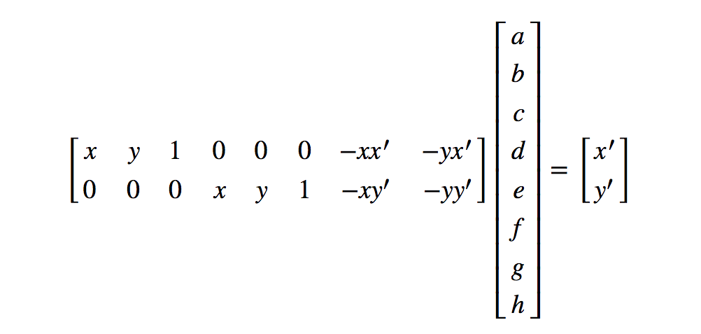
Image Warping and Rectification

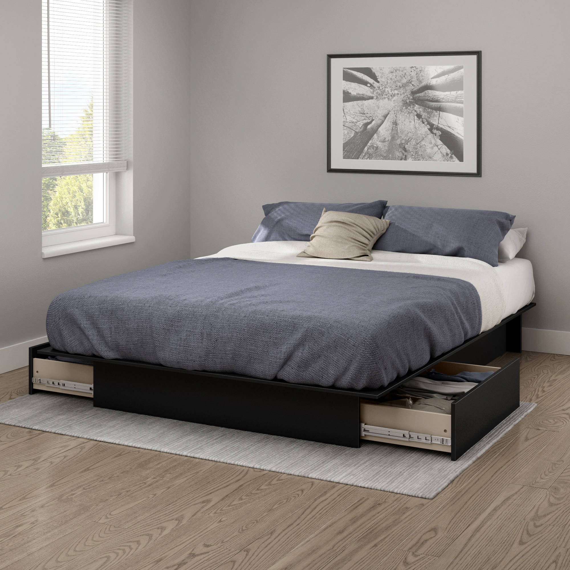
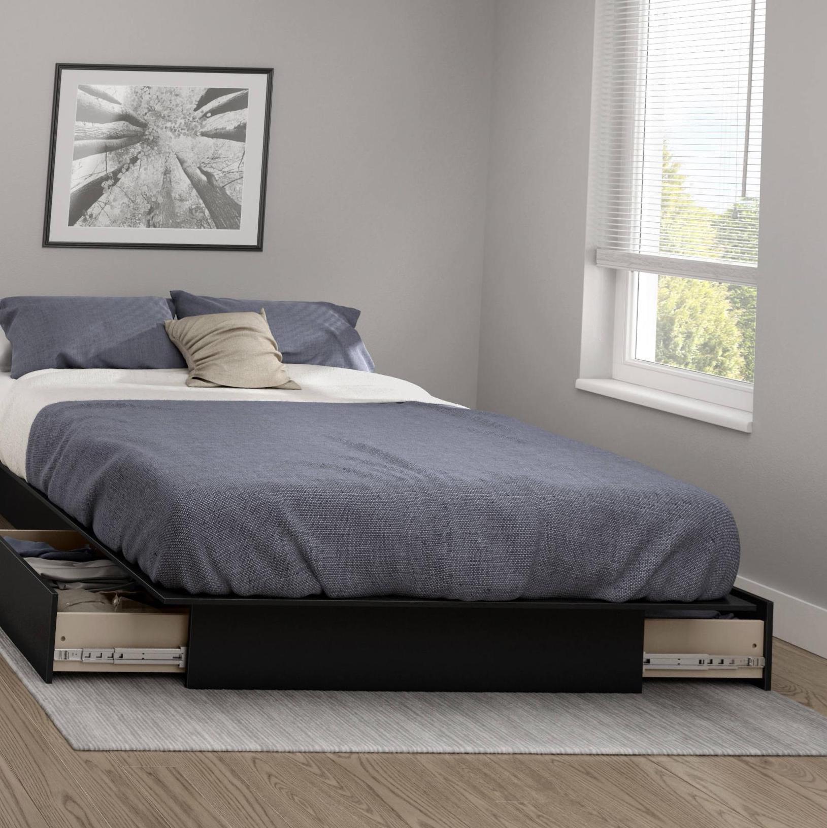
Once the homographies are created, it's time to warp and rectify them. I started by taking a few sample images with some planar surfaces, and warping them so that the plane is frontal-parallel.

For example, I warped this image of a room to the rectangular image frame in the center:

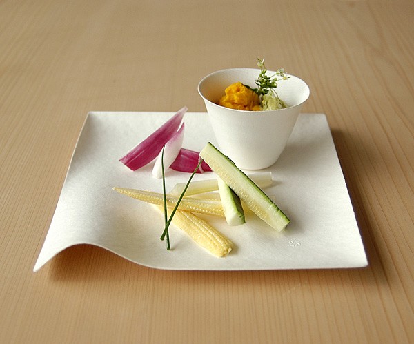
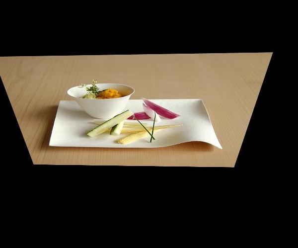
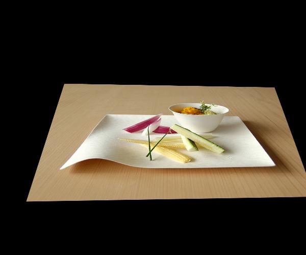
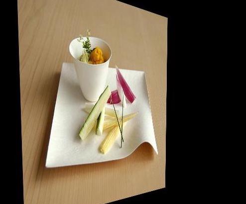
I then tried wraping this plate of food in a bunch of different directions:

With image rectification complete, it was time to move on to the final part, mosaics!

Making Mosaics

Once I finalized my warping algorithm, I began working on creating mosaics of two or more images. I created mosaics by warping two images at once and then warping the resulting image with the next image. I warped the left and right images of the photos I captures onto the plane of the central image in the photos. I experimented with different types of blending. The best results were obtained by creating linear blending over a central region where the two images are combined. I achieved this by creating a horizontal mask (utilizing some of my project 3 code!), spiting the image into distinct color channel and computing a weighted average across the mask's area. My results are illustrated in detail below:

Yellow Meadows

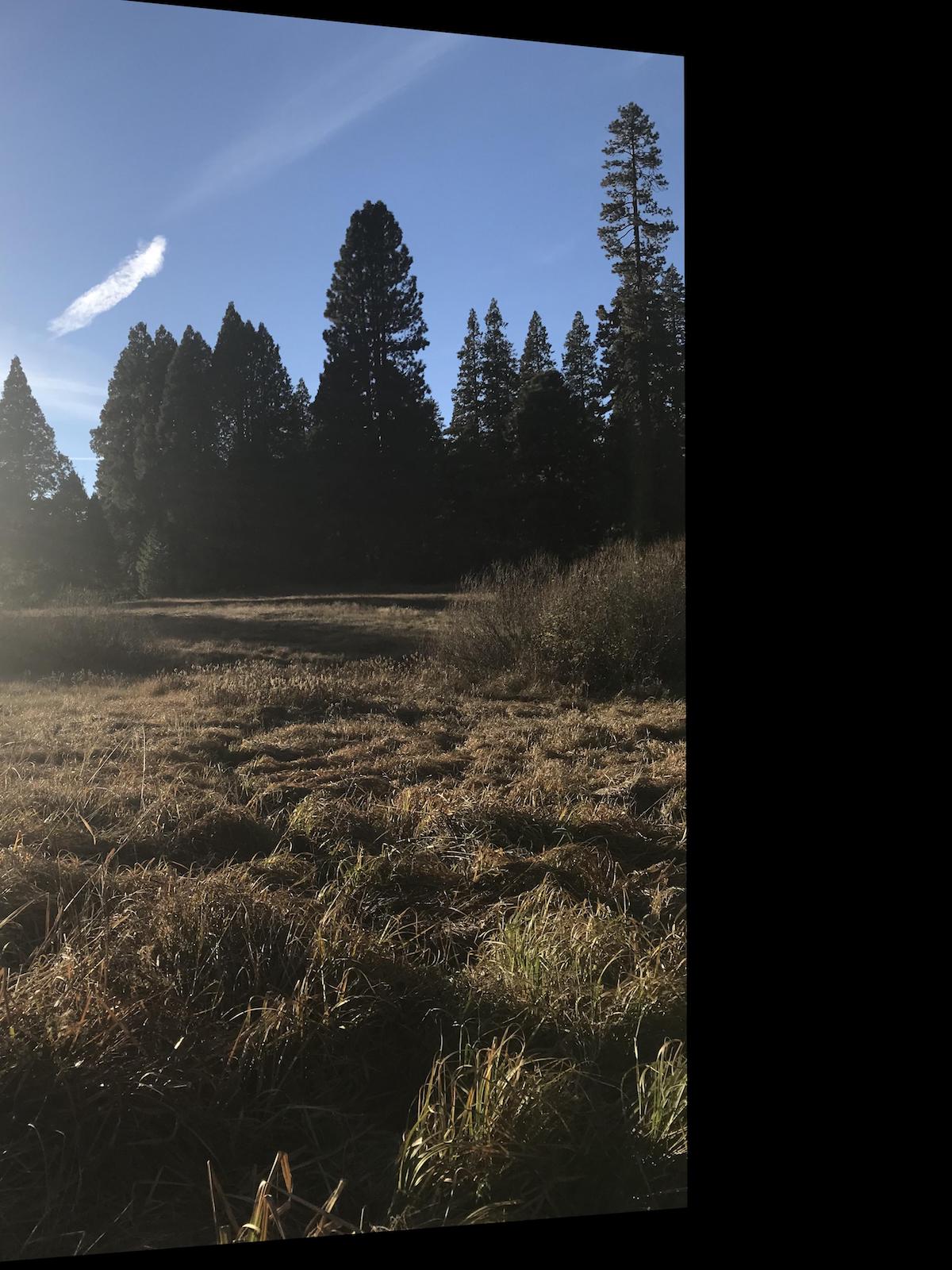
Using these initial images:

I warped the right image into the left image's plane. I found that using more than four correspondence points (between 7 and 11) yielded better blends overall. For this specific set of images, the points of correspondence and the warped image in a new plane are illustrated here:

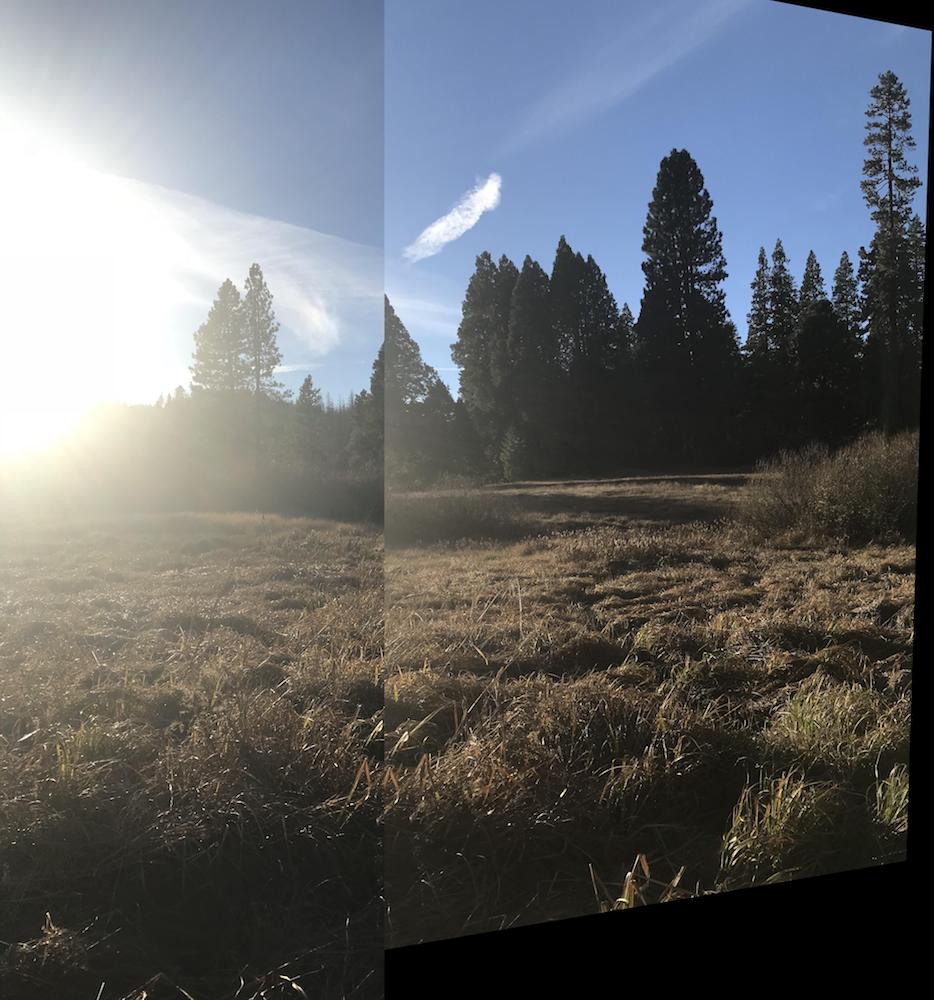
Right image warped to left image's plane

.

With the images in the same plane it was time to put them together:

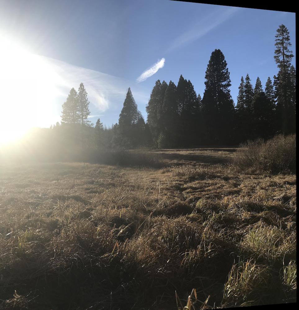
Obviously, this is not an ideal result since the images have different lighting and exposure meaning that the blending is not seamless. To resolve this, I implemented a blending algorithm I wrote in project 3 that involved linear blending across the horizontal plane. The final result looks like this:

Yosemite Forrest

Using these initial images:

I first warped the right image into the middle image's plane. I then also warped left into that resulting image's plane. This way both left and right image were projected onto the middle image's plane.

Second mosaic no blend

Final result with all images blended together
There is a small imperfection in this one at the top of the mountain on the left side that I couldn't get to go away no matter what points of correspondence I used. This results is the most minimal ghosting effect I could achieve but I think it could be further minimized by playing around more with more feature points or window size for blending.

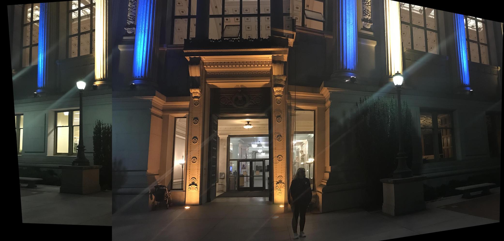
Blue and Gold Lights

Using these initial images:

First mosaic with linear blending

Second mosaic no blend

Final result with all images blended together
There is a little bit of ghosting in this set of images as well that I think could be improved by trying different pixel sizes for the blending window.

Feature Matching for Auto-stitching

In the second part of the project, the goal was to implement an algorithm that can automatically stitch images into a mosaic without having to define correspondence point pairs by hand. To achieve this result, I followed this paper. I detected corner features using a Harris feature detector, extracted feature descriptors for each feature point, and used RANSAC to match feature descriptors between images to produce homographies.
The results are showcased below.

Corner Detection

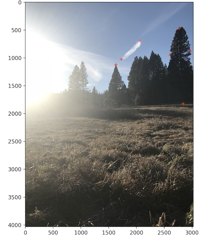
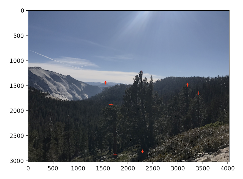
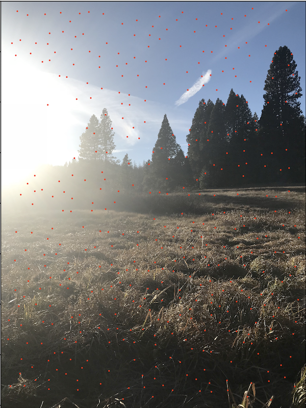
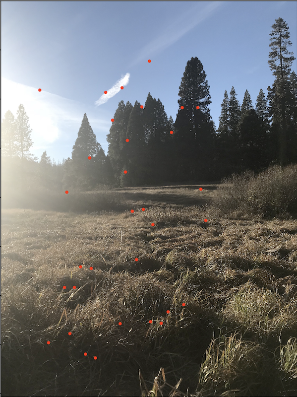
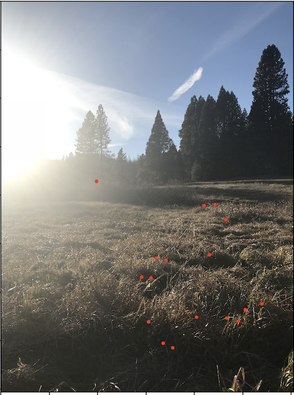
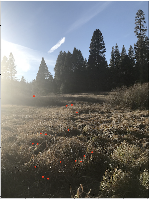
I started by detecting interest points using a Harris Interest Point Detector. The Harris points are measured in their corner response strength. To illustrate the process, I will utilize the yellow meadows photos I used in the first part:

After running the Harris detection algorithm on these images, I got these results. Each red dot designates a corner detected by the algorithm.

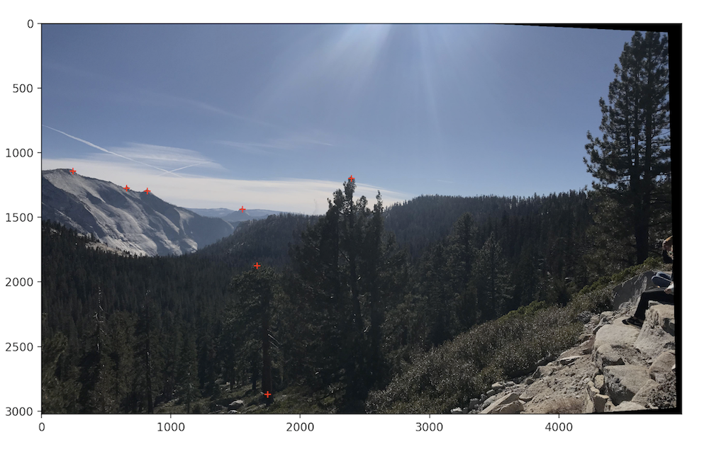
Adaptive Non-Maximal Suppression

The Harris algorithm outputs very many points and some of these points are not as strong as other ones. I used adaptive non maximal suppression to reduce the number of points while also making sure that the points are well distributed across image. I used the approach described in the paper where I calculated r_i values for every Harris point.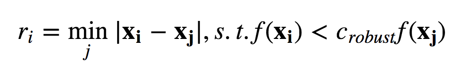

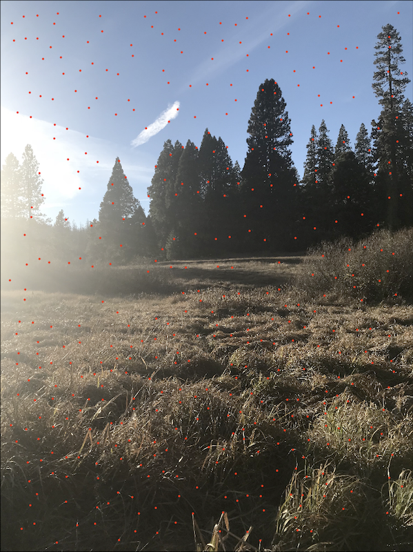
After computing these values, I kept the strongest 500 points. These points have the strongest corner response that are also specially well distributed across the image.

Feature Descriptor Extraction

Now that I had my points of interest, it was time to match them across my images. This can be achieved by creating feature descriptors for each of the Harris points. The algorithm for that is pretty straightforward and includes four steps. First, create a 40 by 40 pixel window centered around each Harris corner then convolve that window with a Gaussian filter. Next, subsample the result from the previous part to end up with an 8 by 8 feature descriptor for that point. Finally, normalize each patch to have mean 0 with standard deviation of 1 to account for bias/gain normalization. This was we are able to reduce the high frequencies around each point and detect matches in the lower frequencies that are resilient to changes in the color intensity between different images. Some examples of enlarged image descriptors I created include: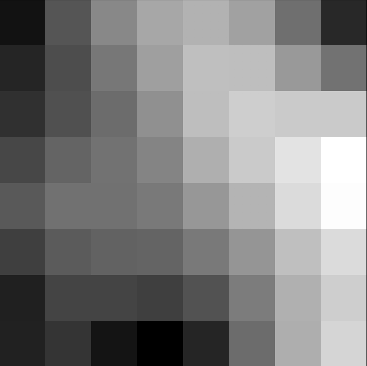

Feature Matching

Once I had feature descriptors for all of my Harris points for both images, I needed to match them. I used a SSD calculation to calculate similarity between pairs of descriptors. In order to reduce false positive rates I followed the approach recommended in the paper which includes the Lower algorithm. I found the best and second best match (1-NN, and 2-NN) for each descriptor. Then I calculated the ratio between these two matches. I set my threshold cutoff point to be 0.3. If 1-NN / 2-NN was below 0.3, it means that the nearest neighbor is significantly better than the second nearest neighbor, increasing the likelihood of a positive match. If that was not the case, I disregarded those points altogether, thus only keeping descriptors that match across the two images. Once I ran this part of my algorithm, I only had the following points left over: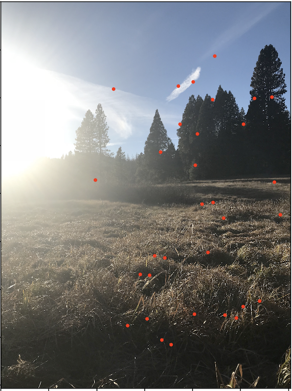

Random Sample Consensus (RANSAC)

Now it was time to compute homographies with the feature matches in place. Due to the fact that there still might be false positive matches after the algorithm above I used the 4-point RANSAC algorithm to reduce the outliers. In this algorithm, a random set of 4 points are selected and a homography is computed based on those points. Then, every correspondence point is mapped from image A to image B using the homography H. Since we know the presumed matches between image A and image B, we can calculate the distance between p_i_prime and H * p_i. I set a metric of approximately 10% as my threshold for what I considered to be a "close enough" match. I then kept all the point pairs that fell within that threshold.

.
I ran this RANSAC algorithm 10,000 times and kept track of the best homography as well as the points that fall below the 10% threshold. I then computed a new homography using all of those points and a least squares computation. This yielded the final resulting mosaics! With the images in the same plane it was time to put them together:

Auto stitched meadow
For comparison, the hand stitches and auto stitched results are displayed side by side:

I think the auto stitched result is actually slightly better, there is a little bit less ghosting going on on the actual blended area. However, in the hand selected image, the homography is less pronounced so that makes the trees look better aligned.

Other Results

Once I finished implementing the algorithms, I recreated the mosaics I made in part one and also made a couple new mosaics. Scroll down to see more of my results!

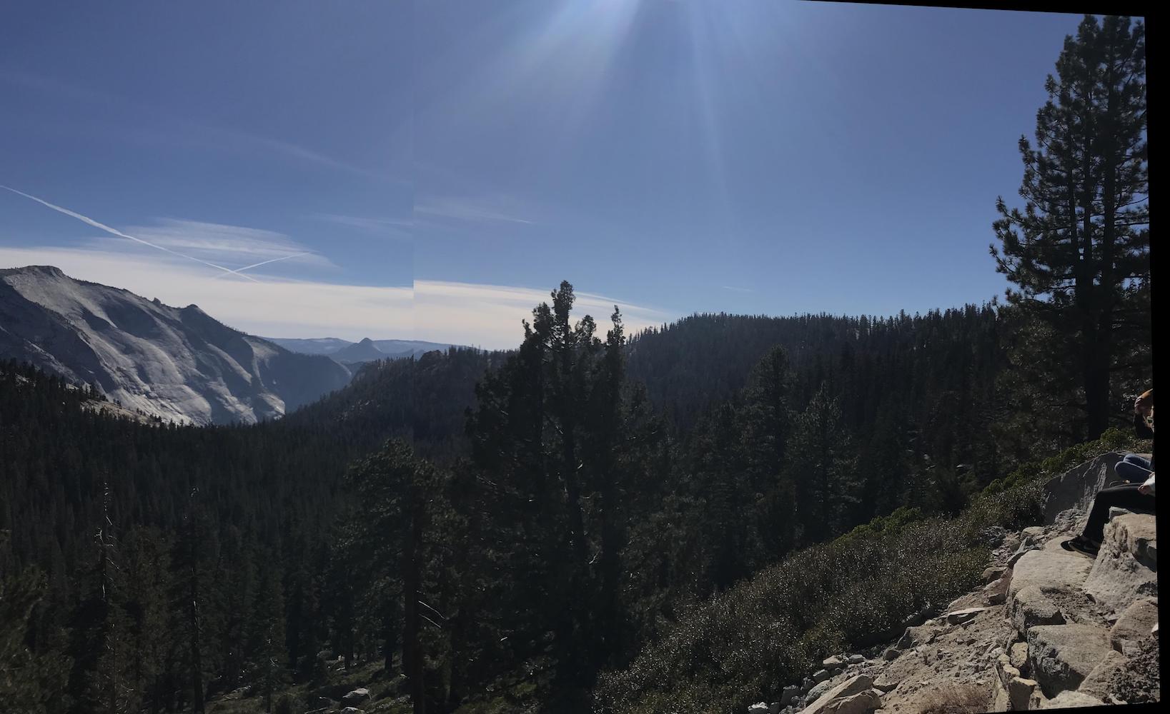
Yosemite Forrest

Auto Stitched -- Forrest

.
I thought the auto stitching algorithm did much better here. There is no ghosting at all! I could not achieve this quality of results with hand selected points despite many attempts.

Blue and Gold Lights

Auto Stitched -- Lights

.
Here the automatic stitching also did much better. The blend is still not perfect however, and I think that has to do with the fact that my point of projection while I was taking these photos with an iPhone camera was not spot on.

Channing Circle

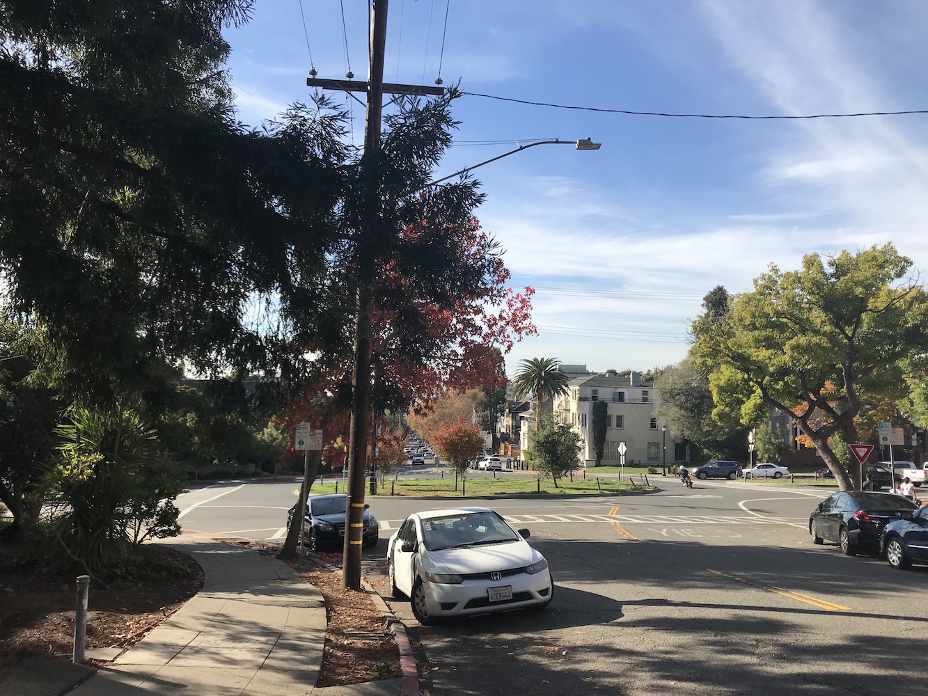
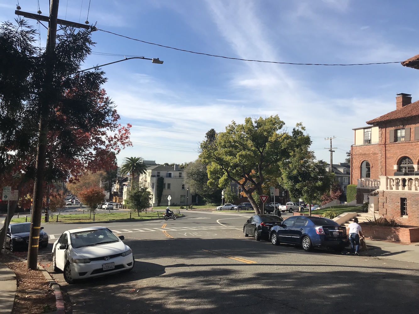
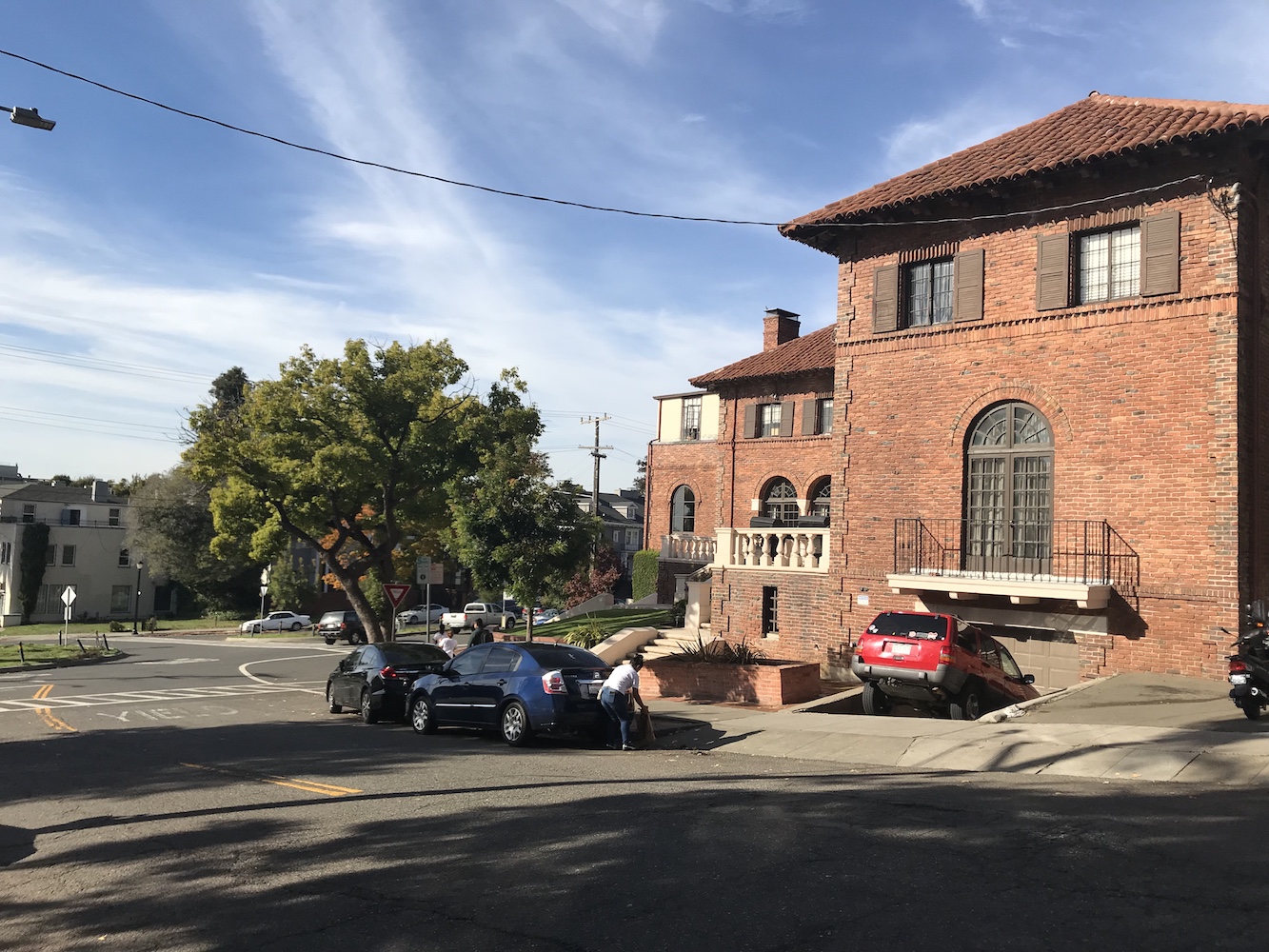
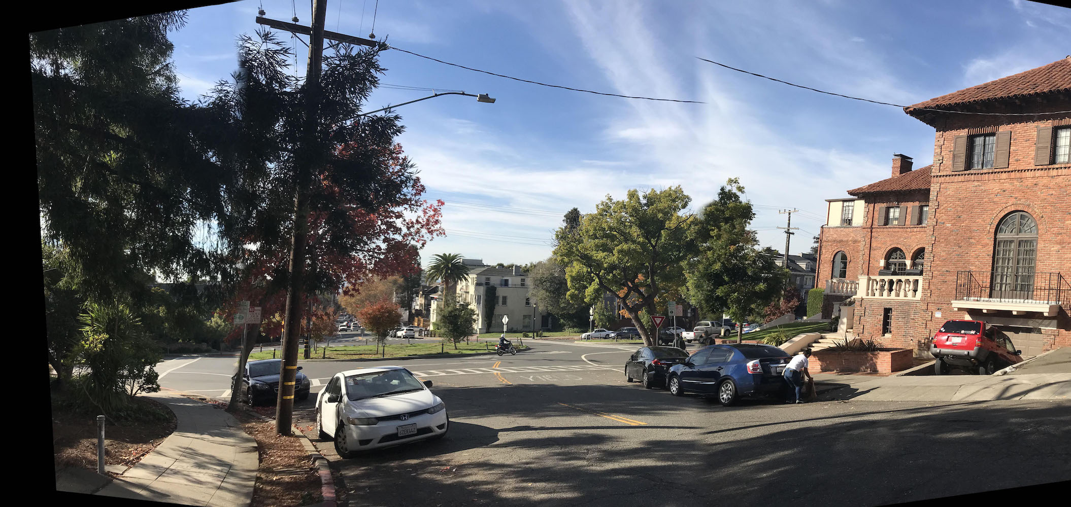
Auto Stitched -- Circle

Bells and Whistles

I thought it would be fun to try my mosaic algorithm on a bunch of different images at the same time by implementing a panorama recognition algorithm. I did this by running my existing algorithms and doing pair wise comparisons image by image. The key modification thought was that after I ran my feature matching function, I counted how many features (or pairs of corresponding features to be exact) it returned. Naturally, if two images are of the same scene, the feature matching algorithm should return many points, while two completely different images should theoretically not align at all. I set a threshold value on the number of features matches that indicate a likely mosaic and only called RANSAC on pairs of images that exceeded that threshold (which I determined about some experimentation to be 14 points of correspondence or more).

Here are the images I started with:

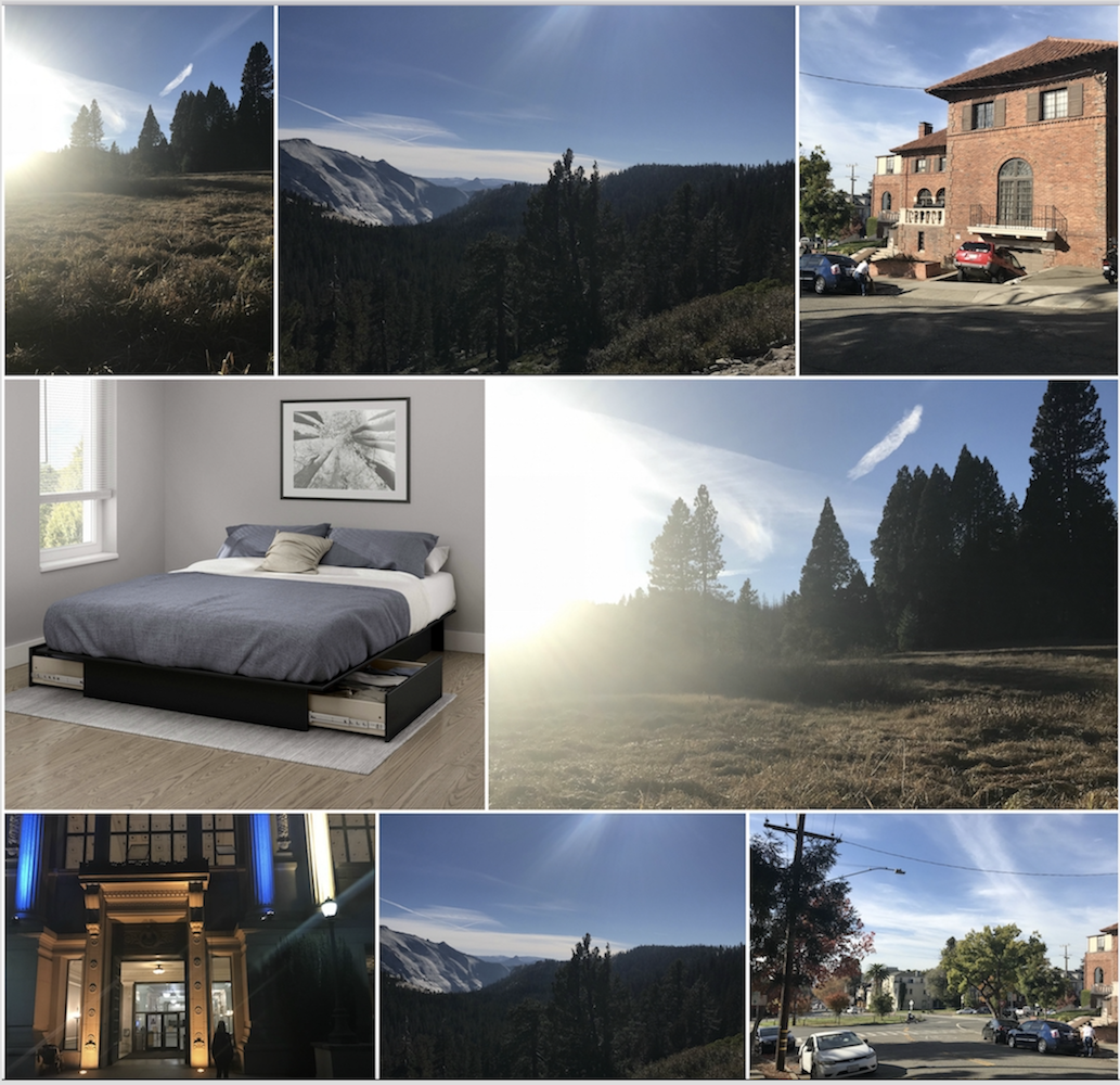
After running the algorithm, I ended up with three mosaics and two individual images:

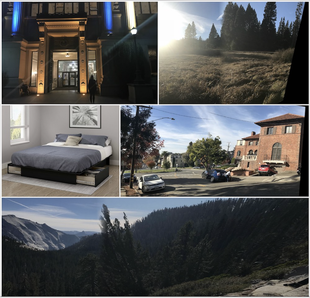
It was really cool to see that with just basic pair-wise comparisons, the algorithm is able to compute correct mosaics!

Final Thoughts

I liked working with large panoramic views during this project and getting to make images even larger and more encompassing. I'm excited about the next part of this project where I will get to experiment with automatically detecting the points of interest.