A) Image Warping and Mosaics

In this assignment, I explore the concept of the $3\times3$ homography matrix $H$. $H$ is used to map augmented points $p=[x,y,1]^T$ to $p'=[x',y',1]^T$. $p'=Hp$. This is useful for aligning two different images of a scene, which were taken at two different perspectives but the same location. Essentially, it can be useful in creating mosaics and panoramas. The matrix $H$ is a combined translation and rotation from one set of coordinates to another. It can be solved, given 4 or more "control points" $(x_i,y_i)$ in each image (points marking the same objects in the two different scenes), through least squares of the system:

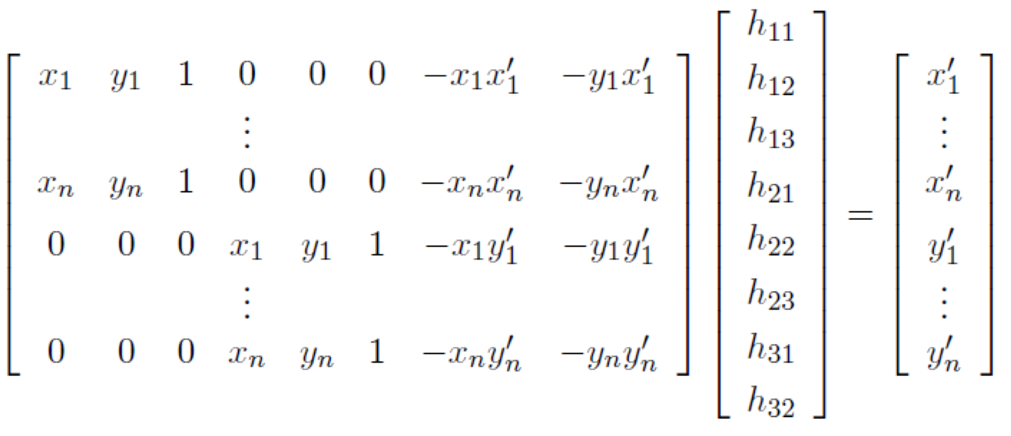
$H_{3,3}=1$ to set a constant scaling factor. After recovering $H$ based on the control points, we can use it to warp one image to be in the same plane as another. Then the two in-plane images can be blended to create a mosaic.

Part 1 - Planar Rectification

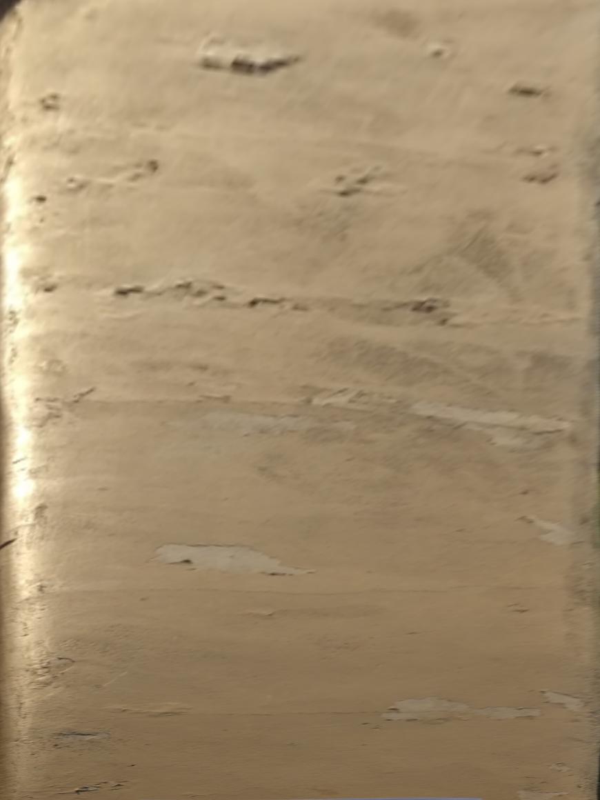
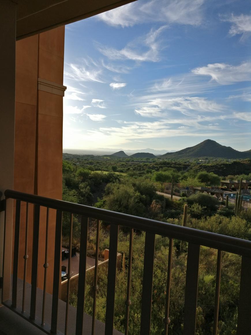
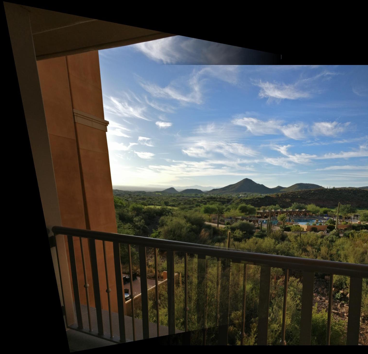
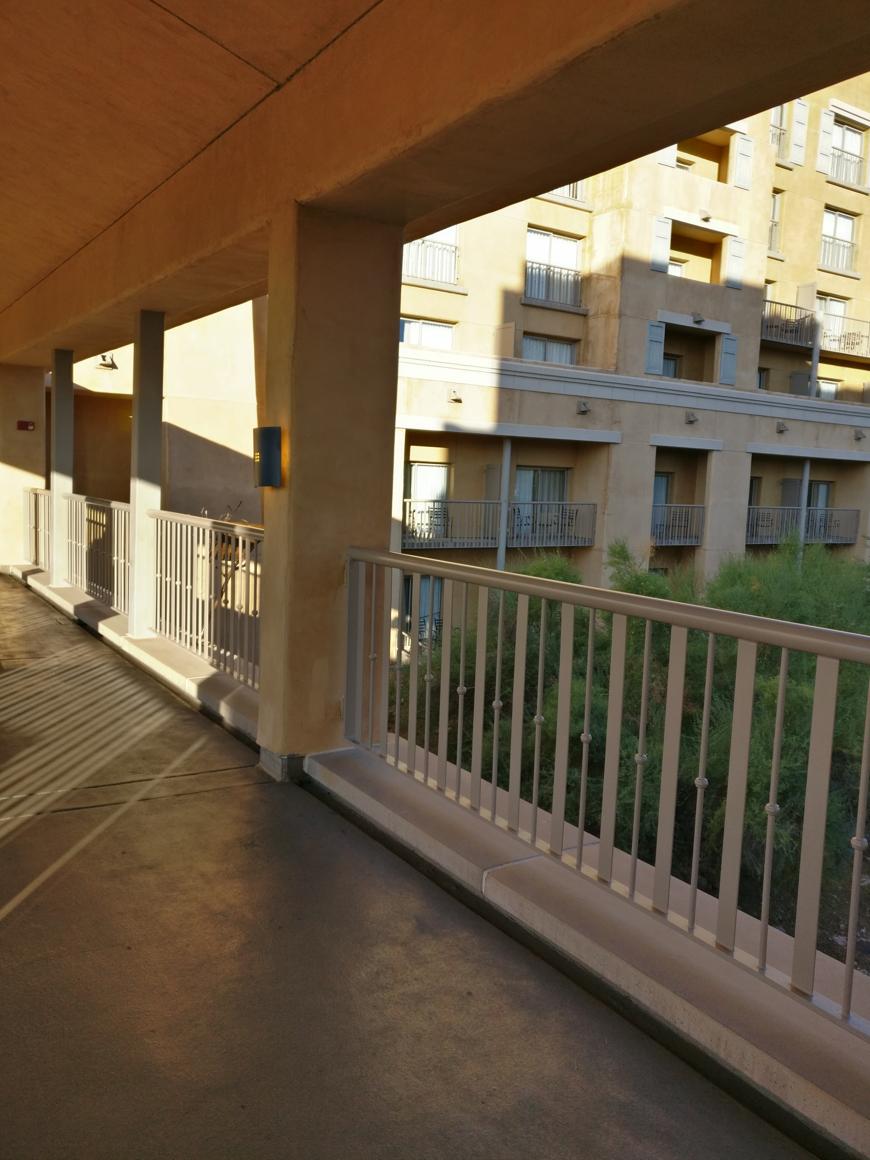
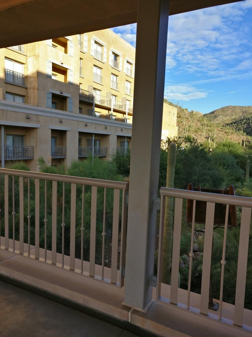
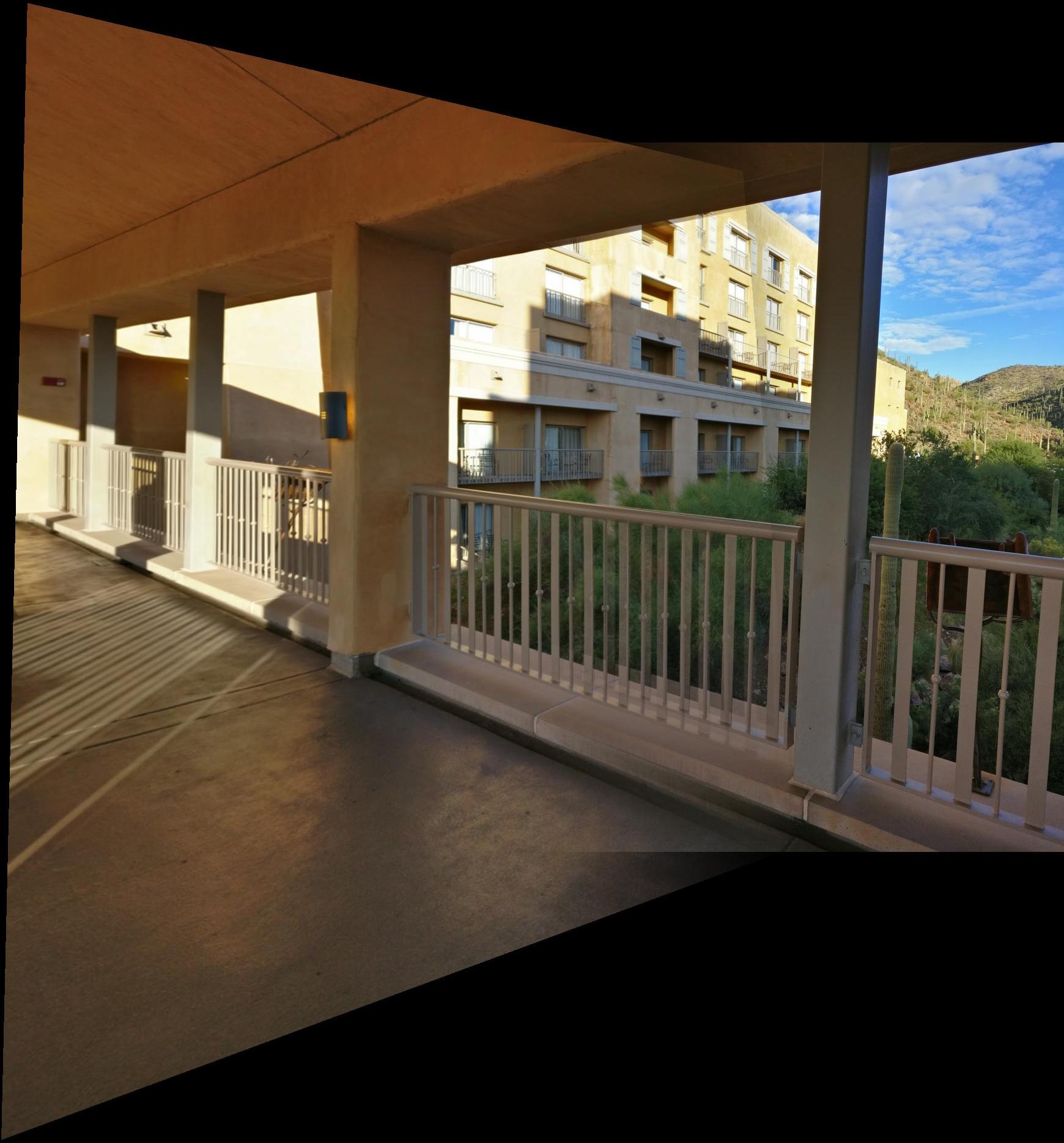
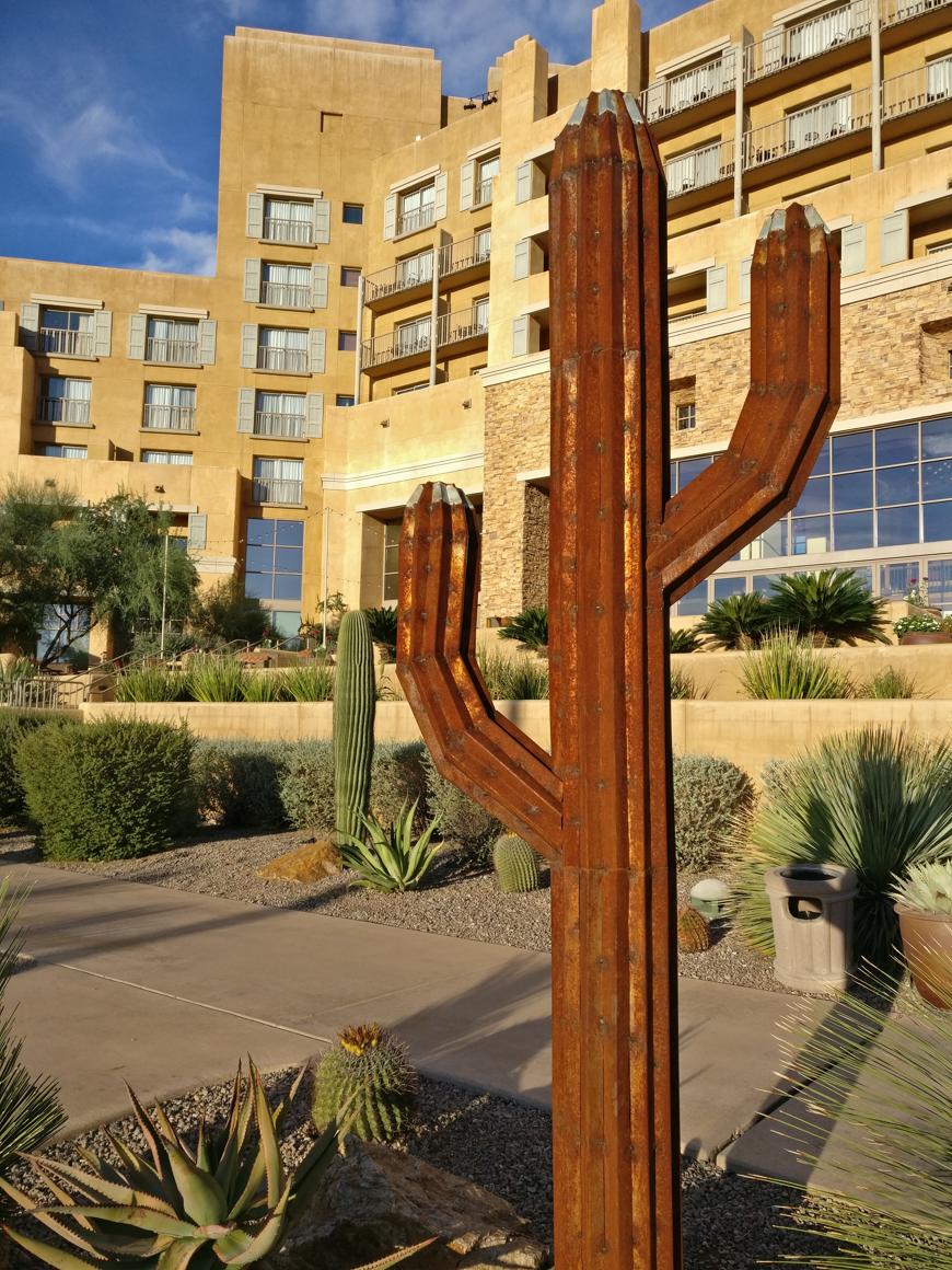
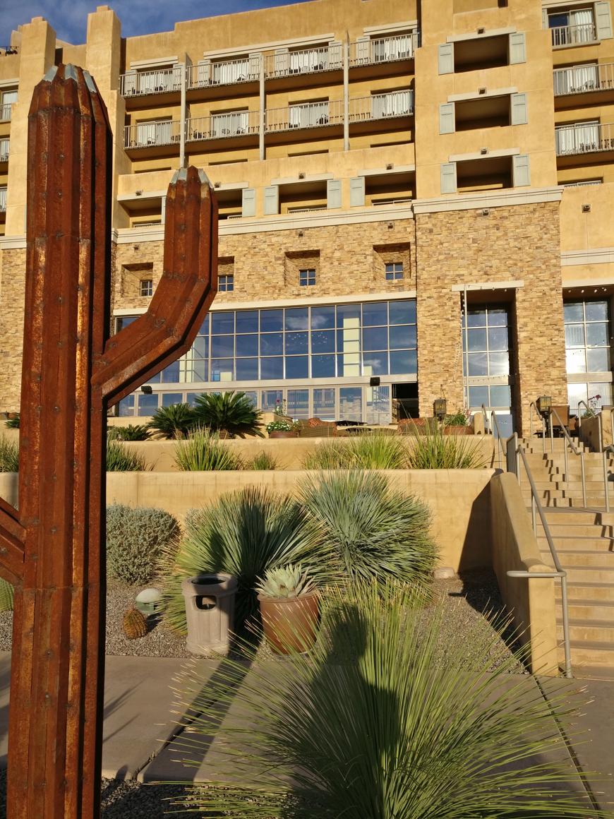
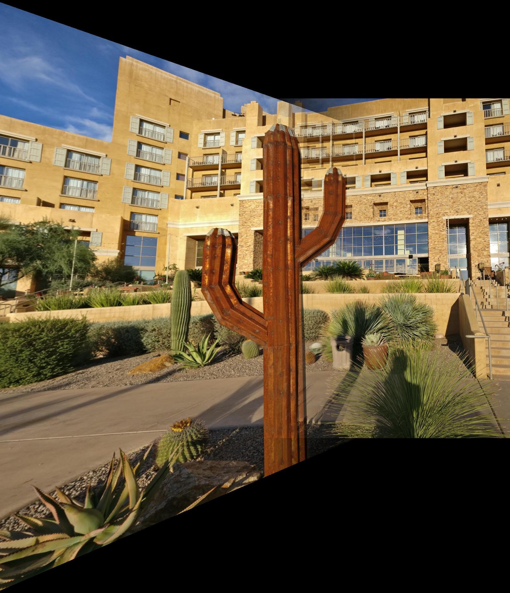
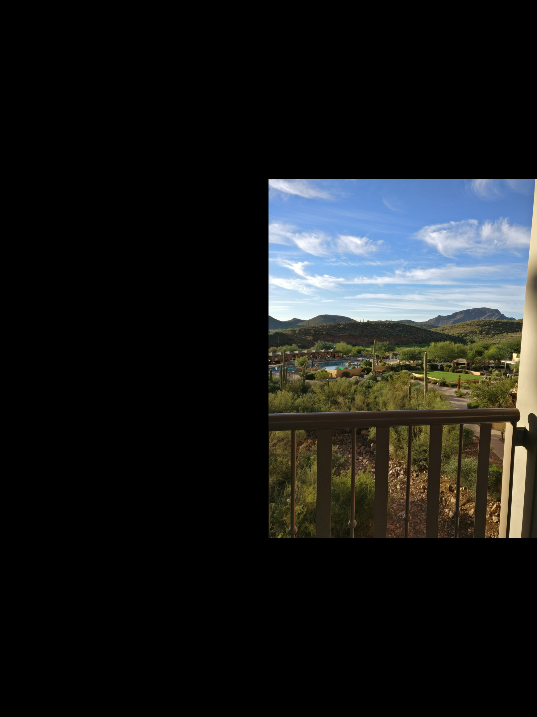
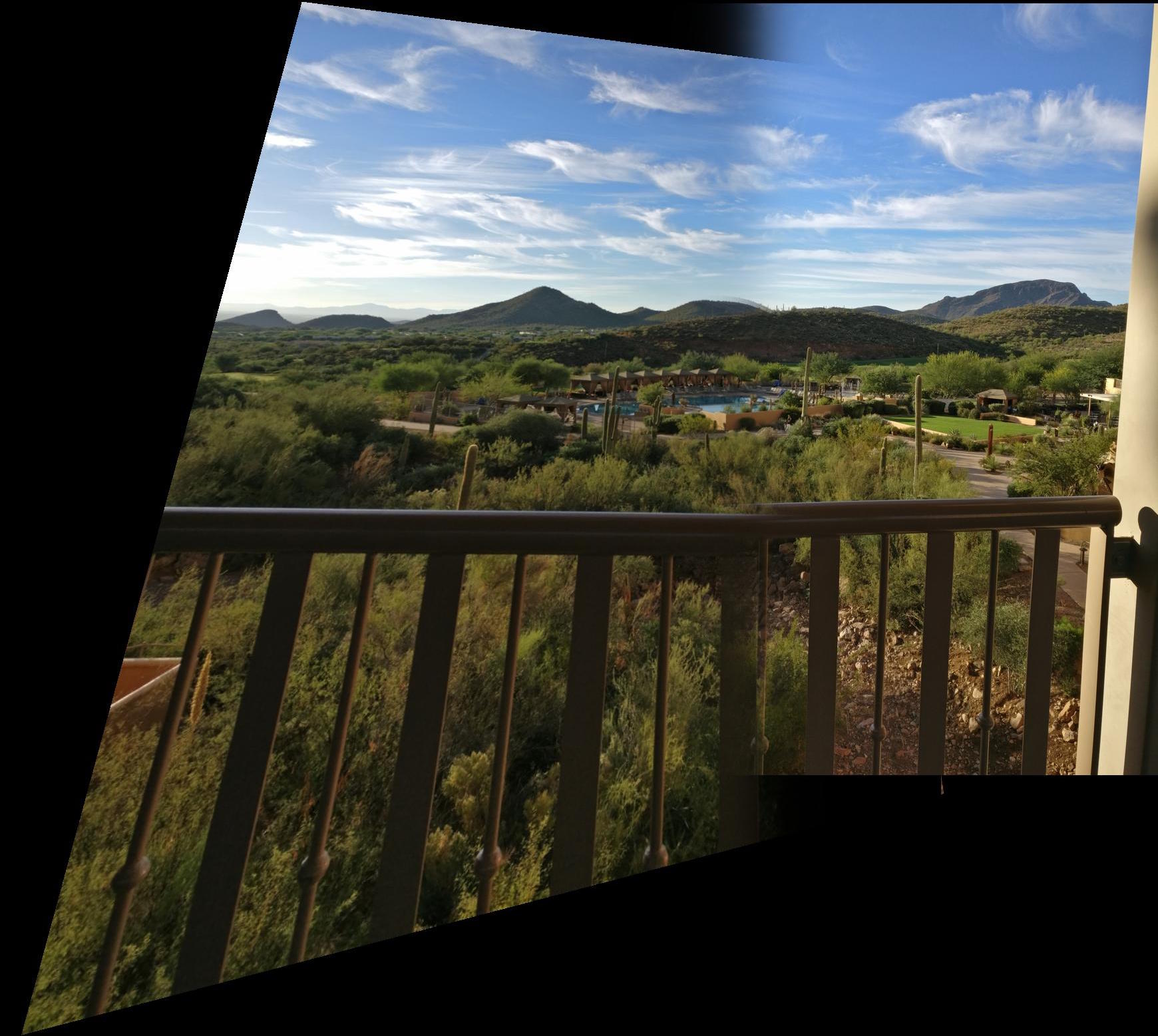
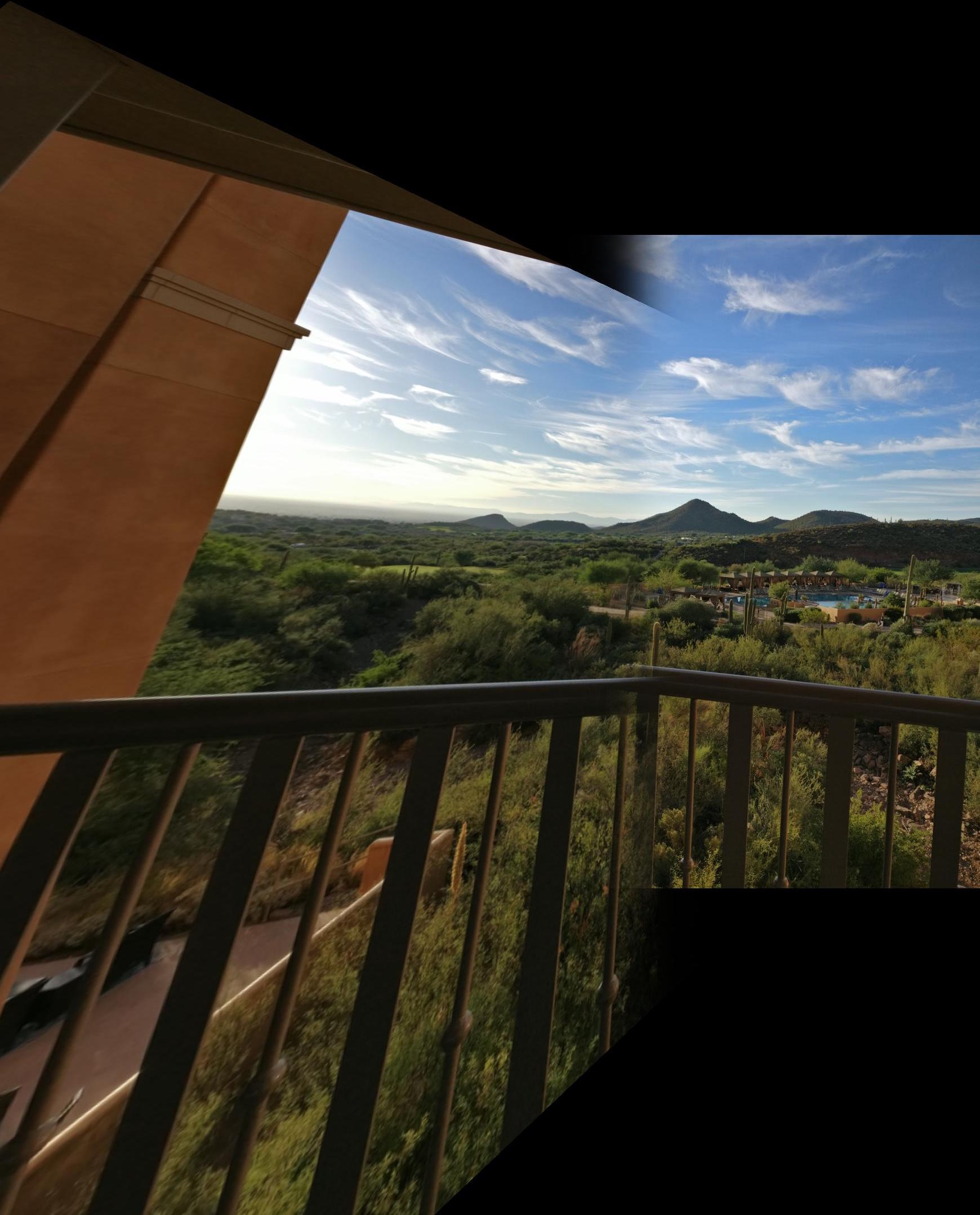
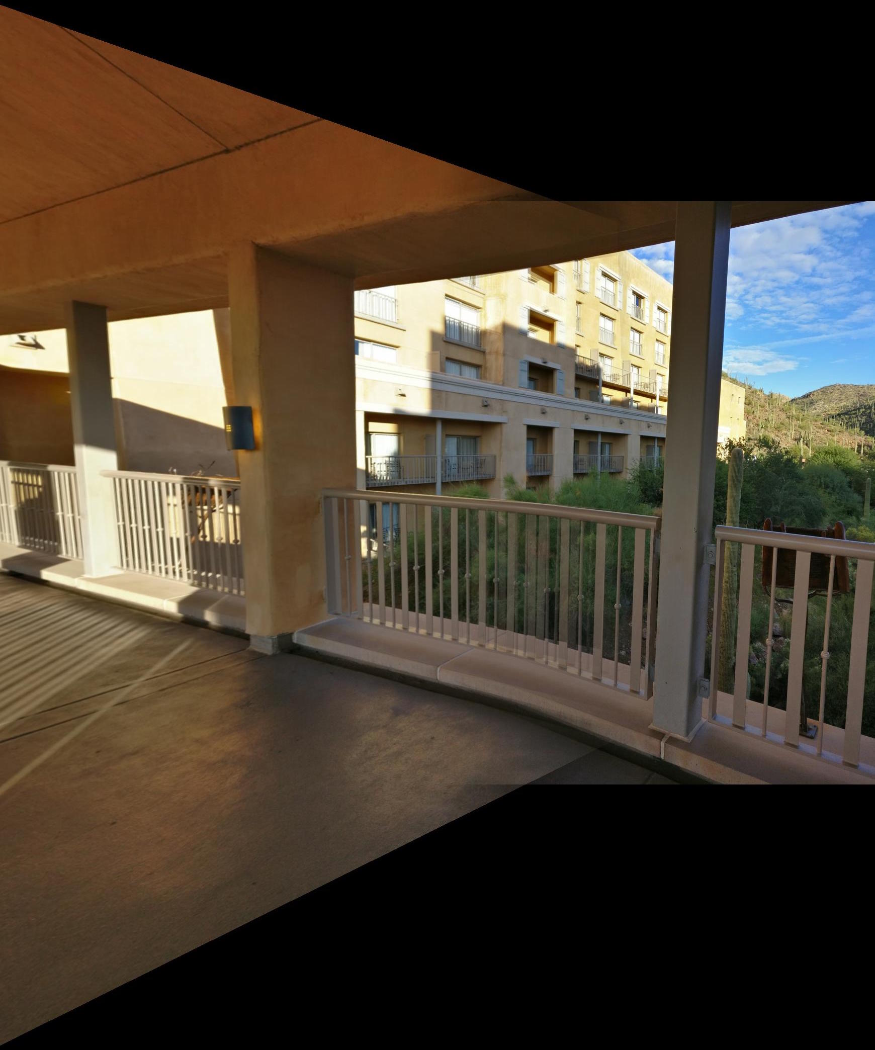
Here, 4 control points are taken from the source image, and the encapsulated quadrilateral is warped using a homography to a regular rectangle. The result is that the normal of the in-image plane points to the audience. That is, the audience looks at the surface from the image face-on and front parallel.

Source Images	Rectified Outputs
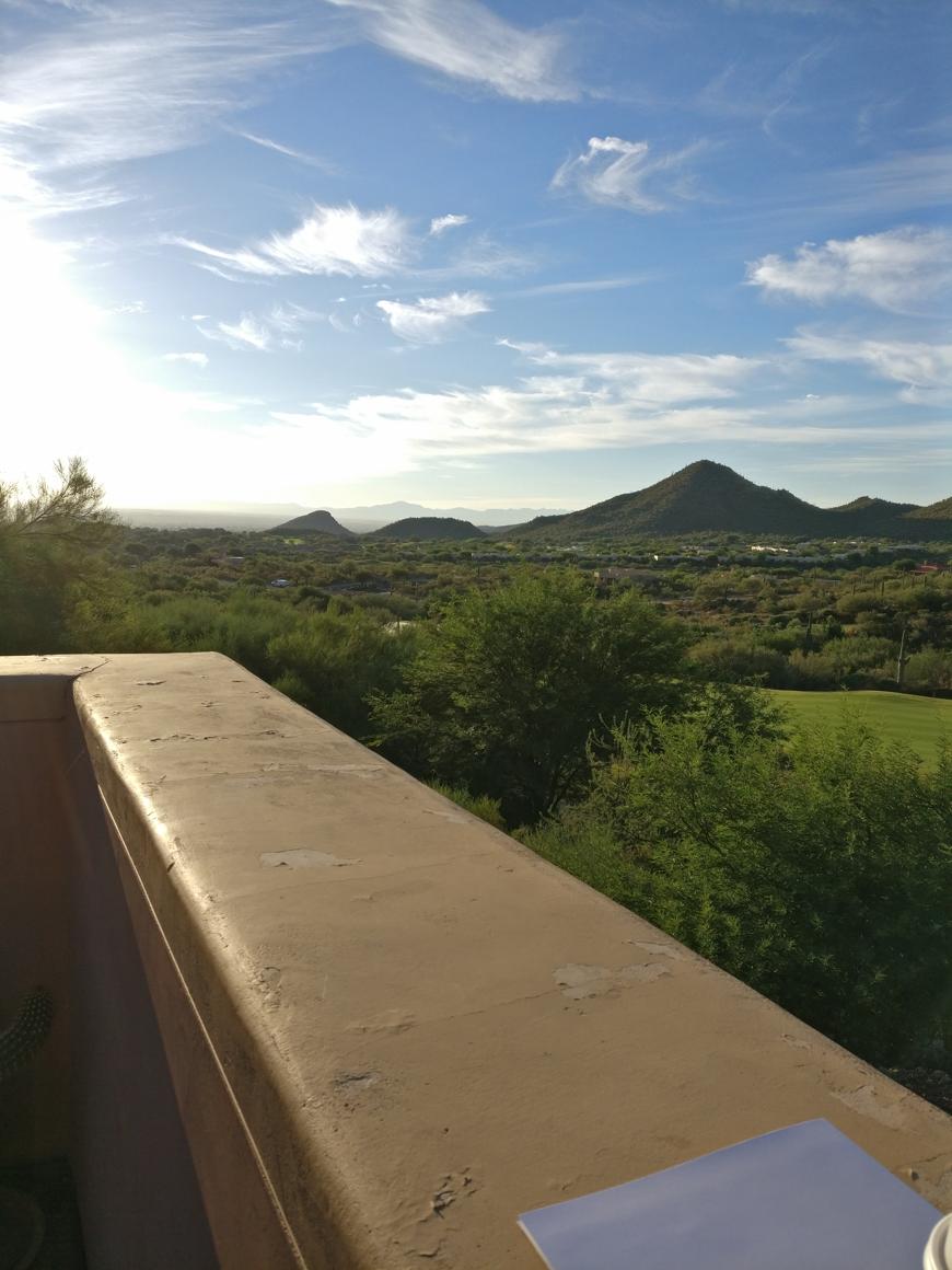
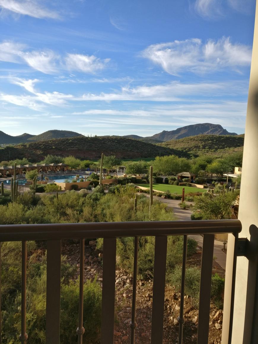
Here, we focus on the texture of the "railing."
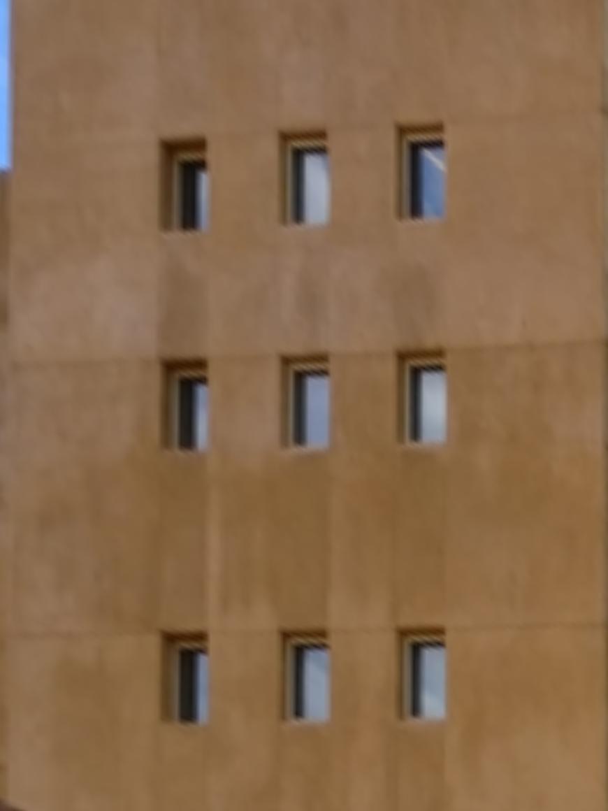
Focusing on the side of the building.
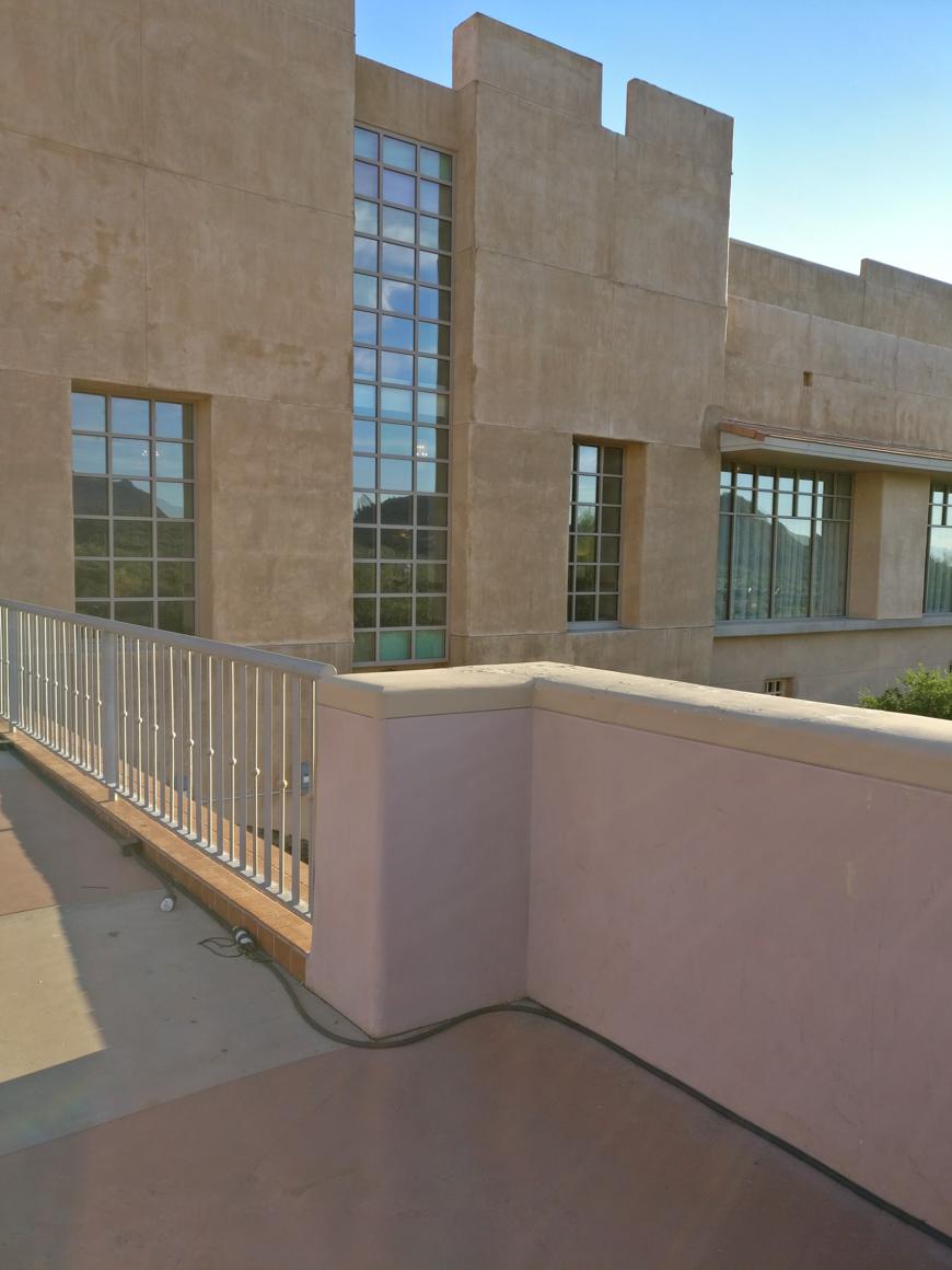
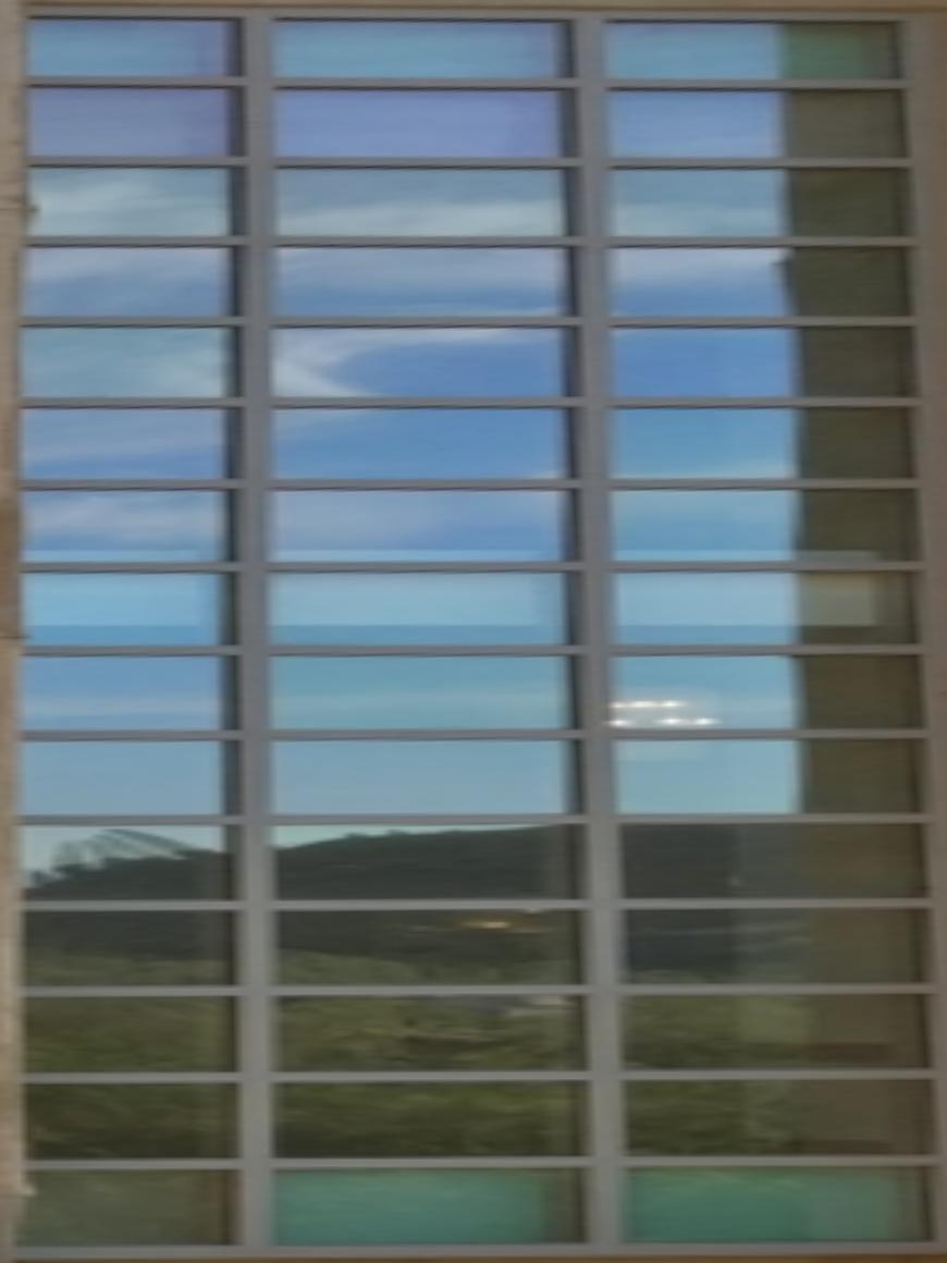
Focusing on the giant glass window.
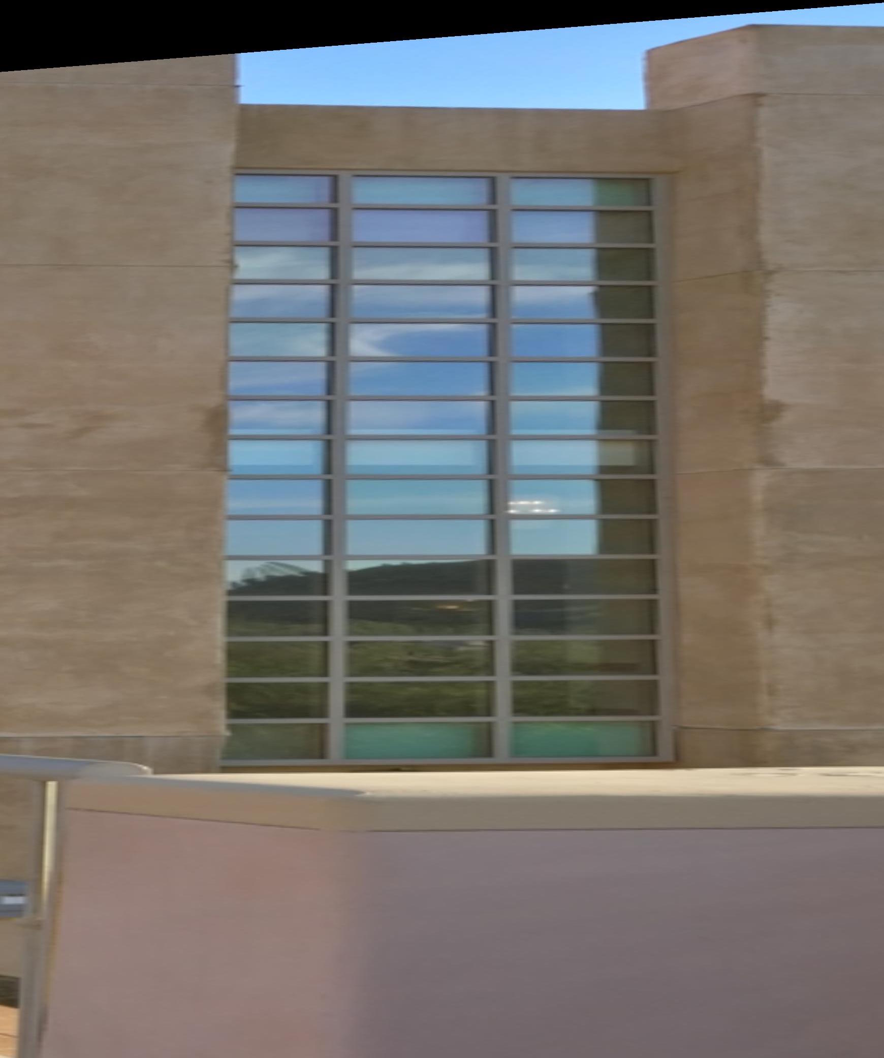
Same as above, but with more of the surrounding scene included

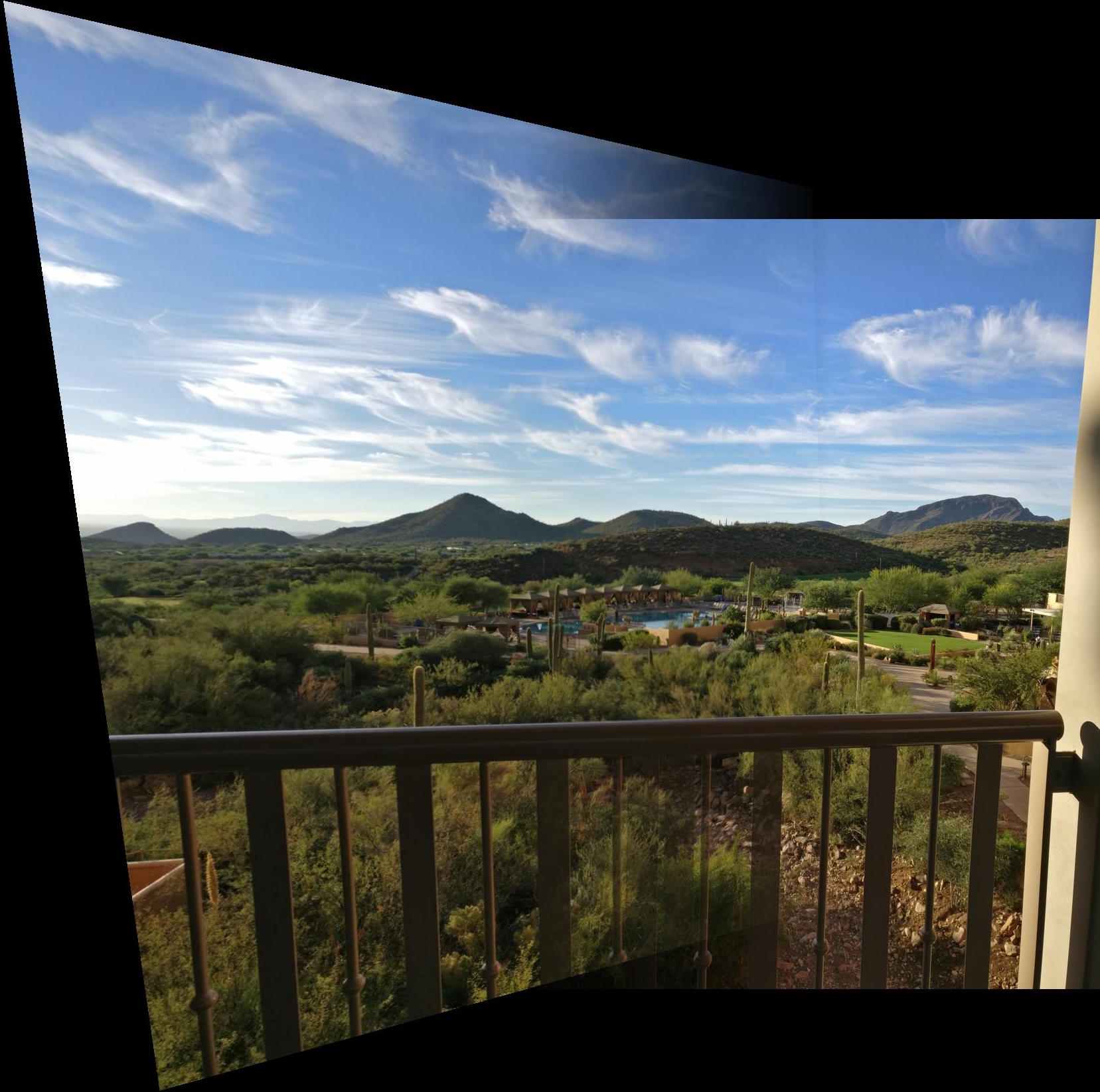
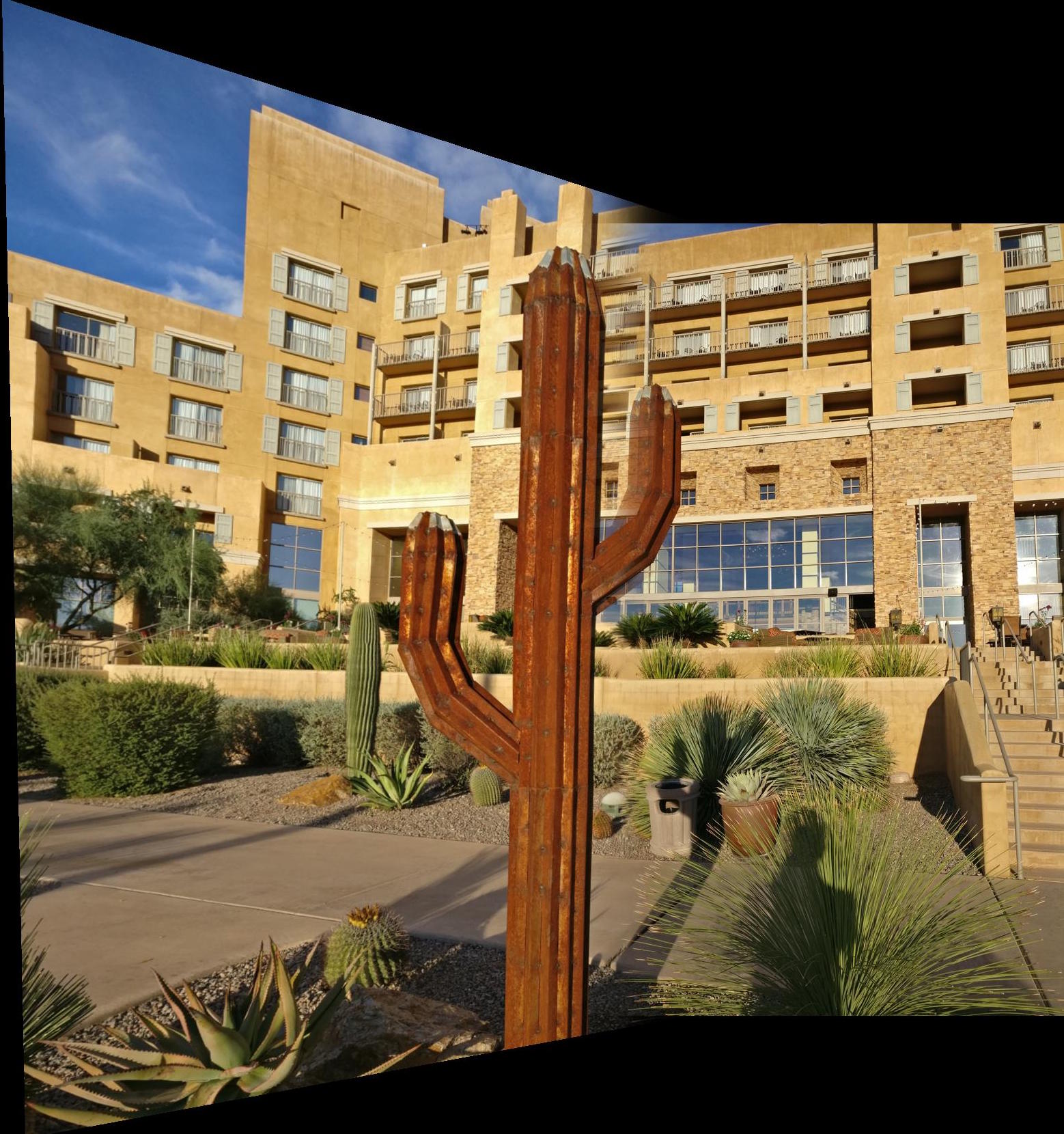
Part 2 - Mosaics

Rather than using a homography to warp to a rectangle, we can use homographies to create mosaics (panoramas)! In this case, we select 4 (or more) control points in two images of the same scene. After computing the homography between the points, we can warp one image to the spatial domain of the other. Then we can blend both the images together to create an output mosaic image. In this case, I used linear blending to combine the input images. The linear blending was used to combine the images so that there wouldn't be obvious seems where the images overlapped. For example, if I simply superimposed the right-hand-side image to the left, the audience would notice a seem where the image met due to slight variances in brightness and color between the two images.

Source Images Left	Source Images Right	Ouput Images

I learned a lot from this project. I found the act of converting a mathematical formula to computer code the most interesting. In mathematical theory, computing the homography seemed relatively simple. Set up $p'=Hp$, then do least squares to solve for the elements in the homography $H$. But when trying to implement that in code, there were several issues that I had to tackle. First, was making sure to double and triple check that all vectors were oriented correctly in Matlab, for the set up of the least squares system. Second, was figuring out how to "apply" $H$ once I computed the homography. It turned out that I need to get the pixels from the base image (right side), apply the homography $H$ to the augmented pixel coordinates, then sample bilinearly from the transforming image (left side). In the math, we want to transform left to right. But to create good images (with no holes or aliasing), we do an inverse tansform and sample. That was a great learning experience!

-----

-----

B) Autostitching

In this section of the project, I implement automatic image alignment and stitching by following the paper Multi-Image Matching using Multi-Scale Oriented Patches” by Brown et al.. Using the paper and some simplifications, I autostitched the previous images as follows:

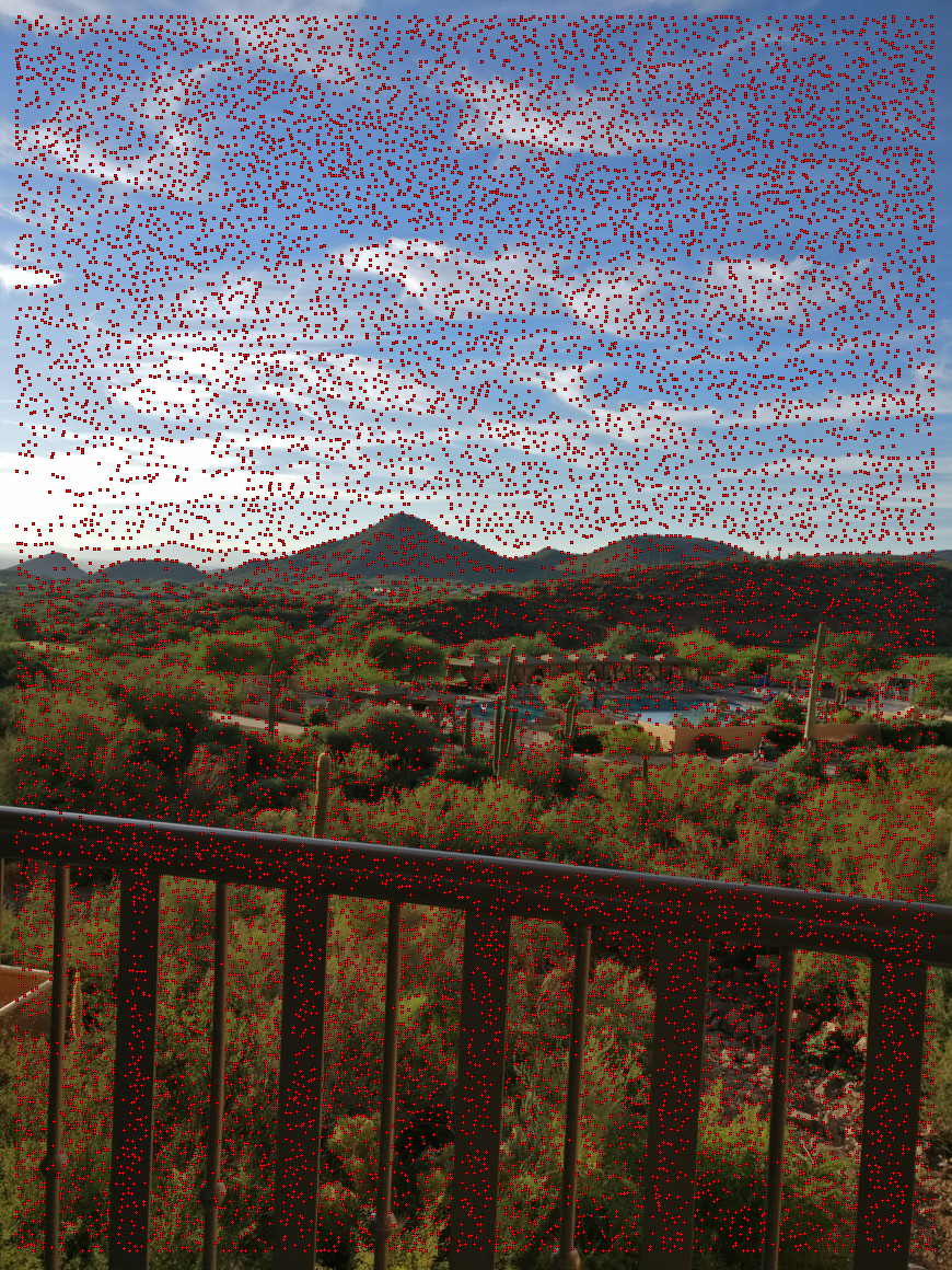
• Use Harris Interest Point Detector to find interesting points, namely corners and edges.
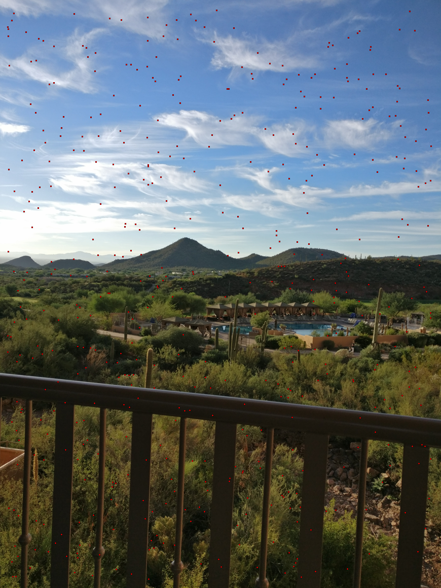
• Use Adaptive Non-Maximal Suppression (ANMS) to obtain better spacing in between interesting points. This prevents clusters of many points within a small area, and allows for non-overlapping feature extraction. That is, so square patches around neighboring points overlap zero or little as possible.
• Extract square patches of features located at the interest points, so that regions of one image can be mapped to another. To obtain a $8\times8$ pixel patch representing a region, I do the following. I first get the $40\times40$ patch of pixels surrounding an interest point. Then I apply a $\sigma=5$ gaussian filter on the $40\times40$ patch, so each pixel contains the information of the neighboring pixels. I then take the middle pixel in each $5\times5$ subpatch in the $40\times40$, and output them to the $8\times8$ feature patch. The $8\times8$ becomes a good, big, and blurred descriptor of a region. Finally, I unroll the $8\times8$ into a $192$ feature vector ($8\times8$ size $\times3$ for each color channel), for future use.
• I then use the Sum Squared Difference technique to find the $1^{st}$ and $2^{nd}$ best match for each region, from the first image to the second. Once the first nearest neighbor and second nearest neighbor of each interest point is found, I reject the pairs of interest points that have $\frac{\text{distance 1-NearestNeighbor}}{\text{distance 2-NearestNeighbor}} < 0.2$. I based this ratio on figure 6(b) of Multi-Image Matching...". This ratio ensures that we only keep interest points that have a great distance from the first closest patch to the next closest patch. Essentially, we want a clear, high distinction between the first closest patch and the rest. Ensuring, we are sure the feature points are good matche/
• Then I use RANSAC to compute a robust homography estimate: (1) Choose 4 points at random. (2) Compute homography. (3) Keep best inliers, removing outliers. (4) Repeat steps 1-3 many iterations. (5) Finally, compute the final homography based on the inliers only.
• Then, I used the least-squares computed homography, and apply it as in the above section with the manual control point selection.

The major benefit of auto-stitching is not having to choose control points. This saves the user a great deal of time and effort. Instead of having to meticously choose spot-on matching pixels and features in separate images, one can simply input the two images and the merge happens fully automatically. However, one downside is that the computer occasionally gets confused and picks poor control points, leading to a good merge in some regions but not the whole image (details below). The error in picking control points can be alleviated using multi-scaling and orienting the feature patches, which were not applied in my implementation. Still, the mosaics turned out well for the most part.

The coolest thing I learned from this part of the project is that we can use statistical approaches to automatically choose control points between two images. Clearly, the individual steps in the algorithm have been researched and developed to a great degree. And the way this paper combines those individual techniques to do autostitching is fascinating. I liked how it was possible to use data from the paper's figure 6(b) to stastically reject vague points, and only keep points we are sure are matching.

Step-by-step (Click to zoom)

	Source Image Left	Source Image Right
Harris Interest Point Detector
Adaptive Non-Maximal Suppression (ANMS)
Top 4 matching points from each image, colored to match. Look around the pool in the image. Two above the pool, one inside the pool, and one on the point of a cactus below the pool.
Autostitch Result

Overall, the manual control point selection is more "visually pleasing." That is, straight and continous lines continue to be straight and continous. For example, notice the hand/guard rail in all of the images. The manual images keep a straight transition, while the autostitching produces a sharp turn where the images meet. In manual selection, humans such as myself tend to select points based on our representation of the object: I chose the corners of the rails, the tip of mountains, the points of the saguaro cacti. The noisy backgrounds seem to just blend together smoothly. In contrast, the automatic point selection based on Harris detection picks based on changes in neighboring pixel data. So it selects locations where it is background noisy, in addition to foreground corners. So Harris chooses some points which are just in the middle of bushes and "blank walls" (seemingly featureless to human perception). The nearest neighboring matching DOES match the noisy points to one another successfully, as shown in the above Step-by-step section. But including them in our RANSAC and least-squares operation produces results that are not as visually pleasing. Yes, the background with the bushes and other flora blend together well, but foreground objects like the handrail is more visually jarring. The main conlusion for me is that manual is more human-visually-pleasing, but significantly slower; and auto-stitching is significantly faster.

Source Images Left	Source Images Right	Manual Control Point Selection	Autostitching