Image Warping and Mosaicing

Zhen Qin

Overview

The goal of this assignment is to perform image warping with a “cool” application -- image mosaicing. I took two or more photographs and create an image mosaic by registering, projective warping, resampling, and compositing them. Along the way, I learned how to compute homographies, and how to use them to warp images.

Part A

Recover homographies

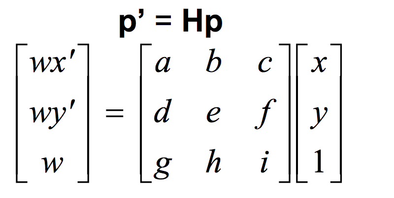
The homography transformation is the same as the following, where H is a 3x3 matrix with 8 degrees of freedom (i is set to 1).



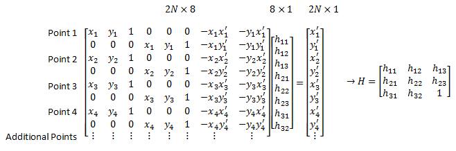
To recover the homography, I select a set of (p’,p) pairs of corresponding points taken from the two images. Then I reformulate the 8 parameters, into the following matrix and use least squares to approximate these eight variables:

Warp the Images and Image Rectification

This step is to “rectify” an image. I took a few sample images with some planar surfaces, and warp them so that the plane is frontal-parallel. To perform this, I first select four corners of the rectangular object in the original image. Then I self define their corresponding target points as a frontal-parallel rectangle and solve a homography matrix to a line-parallel output image. Once the homography matrix is solved, I warp the images using the homography. Here are three results using homography image warping:

Blend the images into a mosaic

For each scene, I took three pictures. Then expand the middle picture as my background image, and warp the left and right pictures into the middle picture. For each wrap, I select 20 corresponding points from each image and compute the homography matrix with least square method.

I use linear blending to blend the left and right image. I first find the overlap part of both image, and perform a linear mask on the over lap part. Then I combine the linear mask with the mask where only right image is nonzero. The following is an example mask the the output image. I find that linear mask behaves very good in this case:

Here are the three pictures from each scene and the final cropped mosaic image

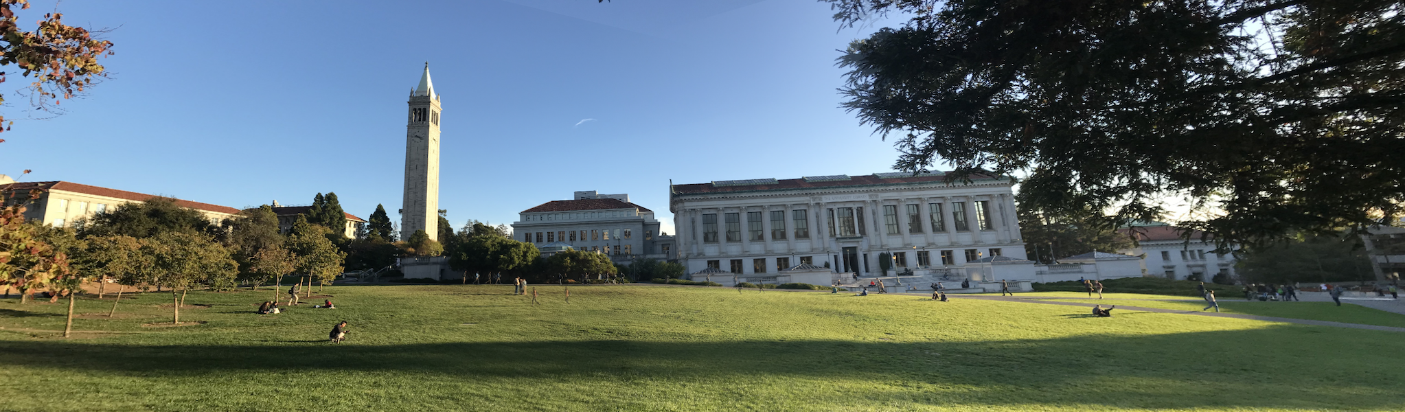
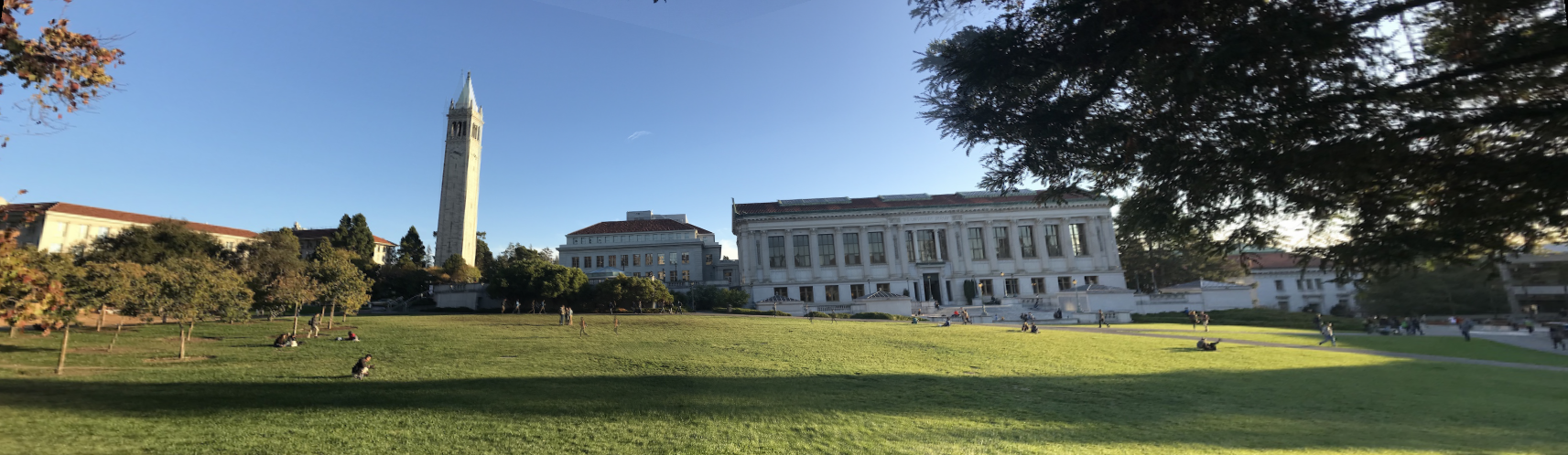
Berkeley Doe Library

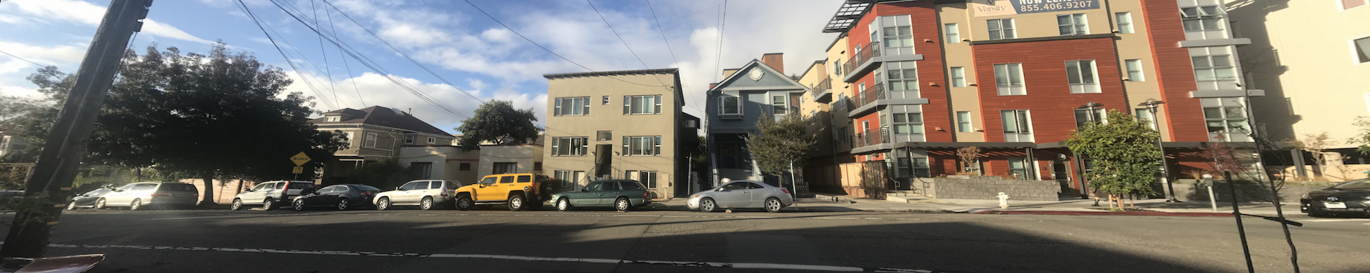
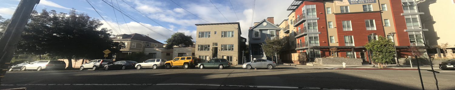
Channing Way

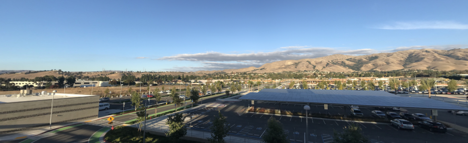
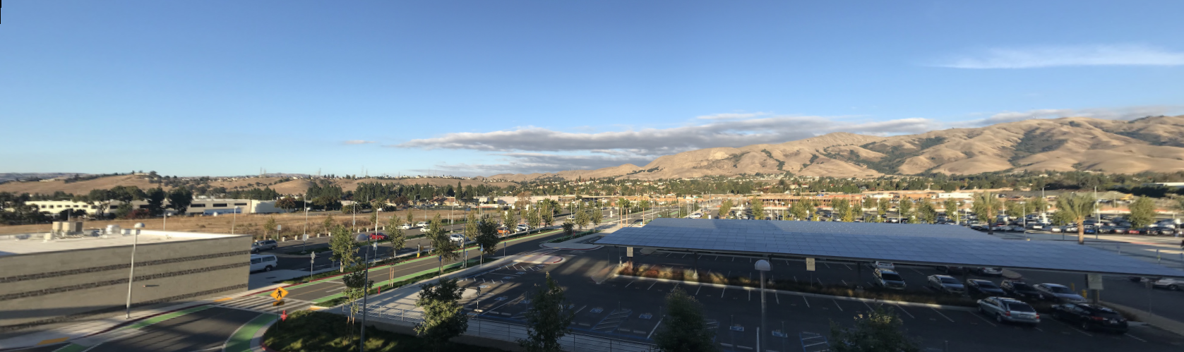
Warm Spring Bart Station

Part B

Harris Interest Point Detector

Corner detection is an approach used within computer vision systems to extract certain kinds of features and infer the contents of an image. In this part of the project we want to auto-detect matching features for Mosaic between two pictures. In the first step, we apply Harris Interest Point Detector, which finds points where both the x and y direction gradients are both substantially large, thereby indicating a corner. Here are harris interest points detected from both left, middle and right images:

Adaptive Non-Maximal Suppression

Harris Interest Point Detector find too many points for each image and we want restrict the maximum number of interest points extracted from each image to save time for computing feature mapping. Therefore, in the second step, I utilized adaptive non-maximal suppression strategy to select 200 interest points from each image. The goal is to find interest points spatially well distributed over the image, since for image stitching applications, the area of overlap between a pair of images may be small.

To implement Adaptive Non-Maximal Suppression Algorithm, for each point detected by the Harris corner detector, we radiates outwards until another Harris corner with a score greater than 0.9 the original point's value is found. The distance between the center and this point is our maximal radius. We then take the top 200 points with the greatest maximal radius.

Here are the 200 points selected after Adaptive Non-Maximal Suppression from both left, middle and right images:

Feature Descriptor extraction and Feature Matching

In this step we want to roughly match all the feature points from each image. First, we represent a feature point detected from last step with a 40x40 patch of pixels centered at this feature point. Then I smooth it with a Gaussian filter, and downsample it to get an 8 x 8 patch. Then I normalize the patch across all color channels. The picture becomes darker after normalization but the overall matching is improved after normalization. Here is an example corner patch after the steps described:

Then I keep all the color channels of this 8 x 8 patch to get a normalized 3*8*8 length vector to represent each feature point. I computed SSD as the distance between every two possible vector matchings. I find the distance of first nearest neighbor and second nearest neighbor as 1-nn, 2-nn and used 1-nn/2-nn distance as a metric to select potential matches. I used a threshold value of 0.5 such that only vectors with 1-nn/2-nn > 0.5 would be matched with their nearest neighbor. Here are the result matchings:

Random Sample Consensus (RANSAC)

After the previous steps, it’s possible that there are mismatching feature points. So in this final step we apply Random Sample Consensus (RANSAC). RANSAC introduces a stochastic method to find homography and thus is very efficient. Here is the algorithm:

RANSAC Loop:
1. Select four feature pairs at random
2. Compute homography H (exact)
3. Compute inliers where SSD(pi’, H pi) less than ε
4. Keep largest set of inliers
5. Re-compute least-squares H estimate on all of the inliers.


I repeated the loop for 1000 iterations, and set the threshold for inliers as 2 pixels. Then I get the following matchings:

Automatic and Manual Image Alignment Results Comparison:

After find all the corresponding features points automatically, we compute the homographies matrix, warp and blend the images with same approach. Here is the comparison of Automatic and Manual Image Alignment Results:

Manual:

Automatic:

Manual:

Automatic:

Manual:

Automatic:

Reference

HTML/CSS for this page was taken from https://v4-alpha.getbootstrap.com/components/card/