[Auto]Stitching Photo Mosaics
CS 194-26 Project 6
cs194-26-aek
Introduction
In this project, we explore how to rectify photographs and create image mosaics by applying projective transforms (homographies) and stitching the resulting images together.
Table of Contents
Part A: Image Warping and Mosaicing
Defining Correspondences
First, we have to define point correspondences between the two images. We can do this using the ginput to select points on the source image and points on the target image. We will need to select more than four pairs of points, since we are solving for 8 unknown entries of the homography matrix H. Using these points, we can recover the homography matrix that allows us to warp one image onto another.
Recovering Homographies
In order to perform projective transforms on images, we need to recover the parameters of the transformation between each pair of corresponding points. The parameters are expressed as a 3x3 homography matrix H:
Warp the Images
Once we've recovered the homography matrix H, we can warp the images using inverse warping. First, we must calculate the resulting image's corners by taking the original image's corners and applying the warp to those points. Then, we can take the inverse of the homography matrix to construct the resulting image.
Image Rectification
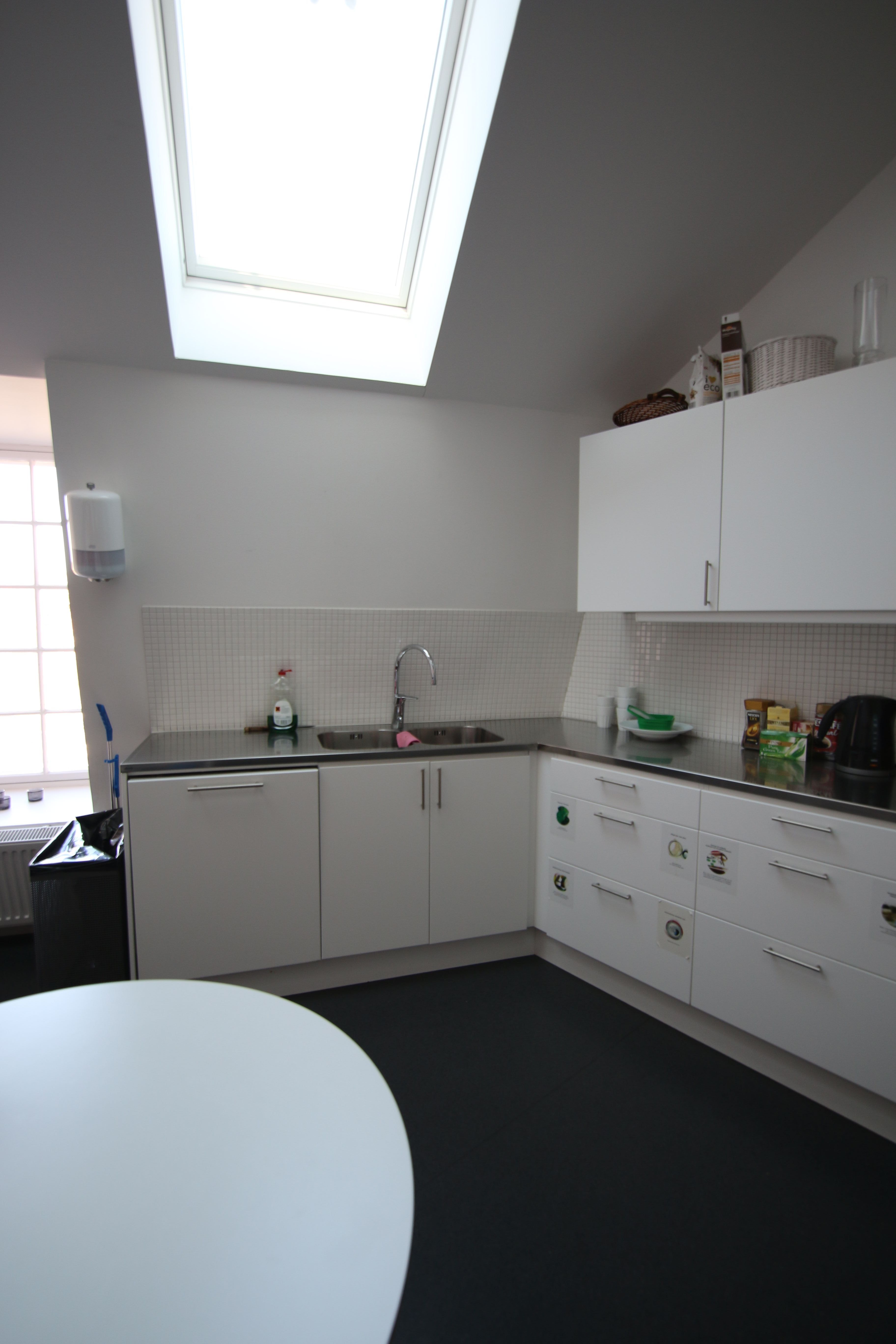
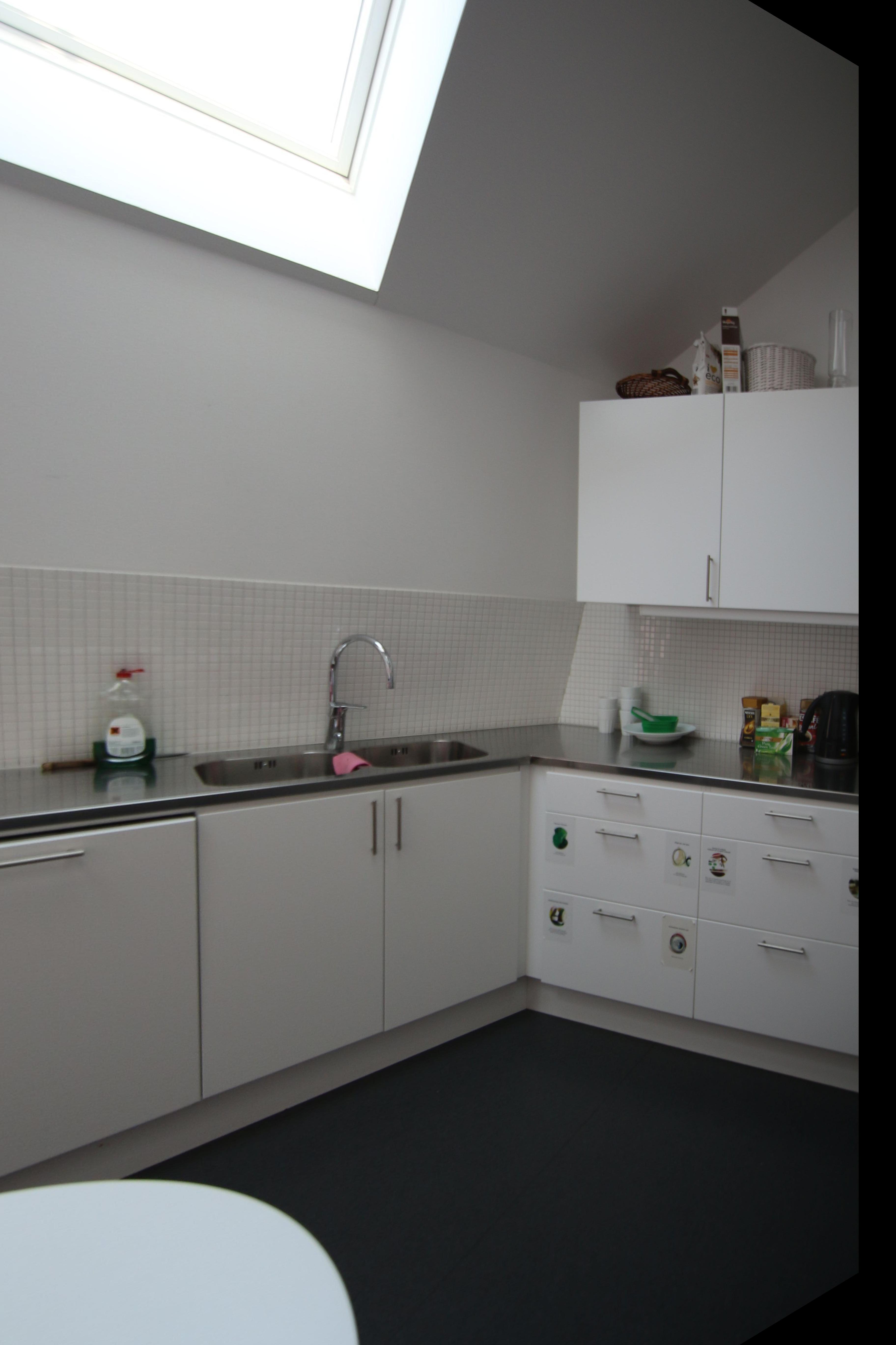
Using the homography and warping techniques described above, we can warp images taken from a viewpoint into an image taken from a different viewpoint. We can do this by creating a point correspondence using a known shape in the original image (in this case, a window or a painting), and rectifying those points so that the resulting image will be head-on. The results are below.
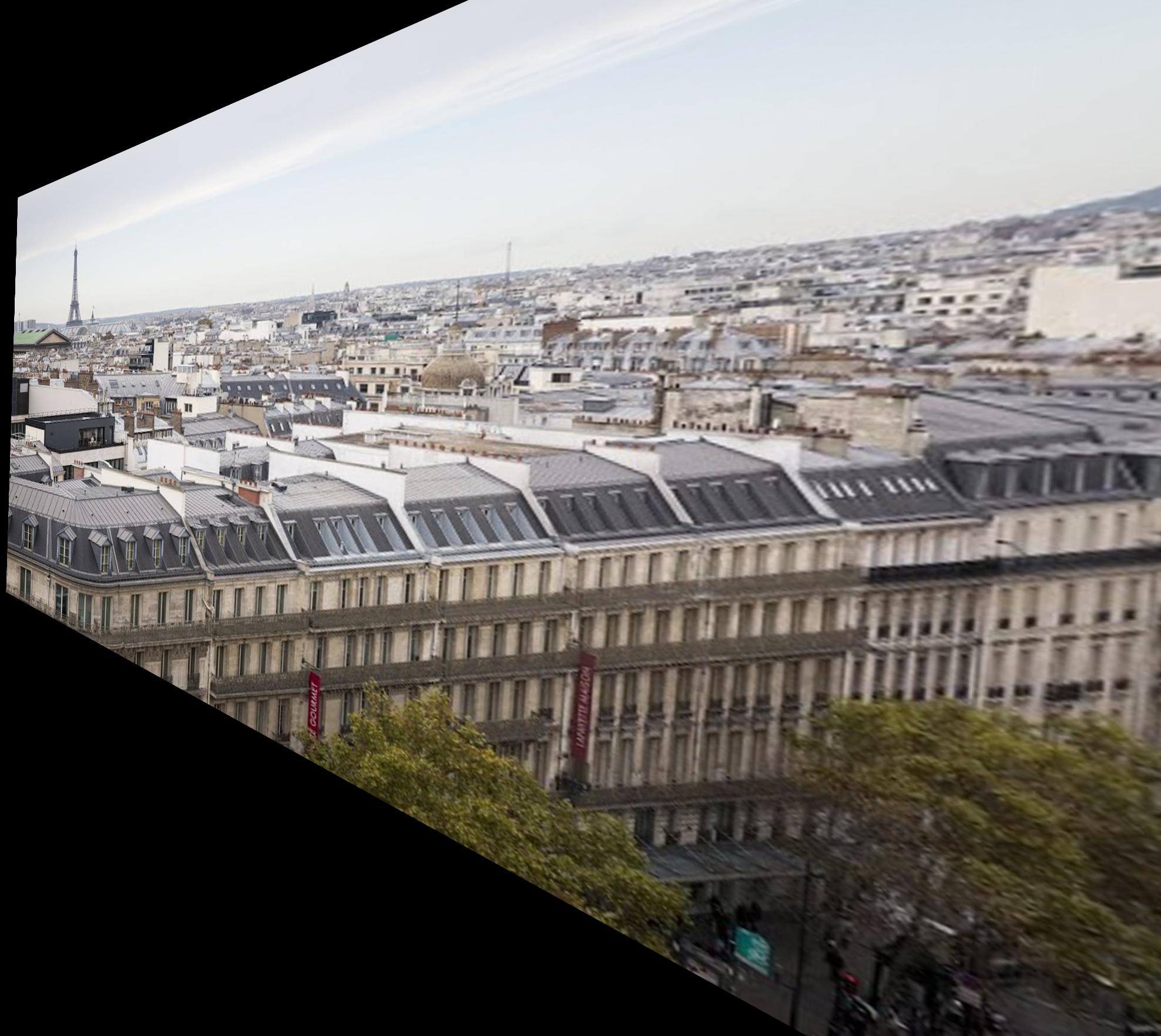
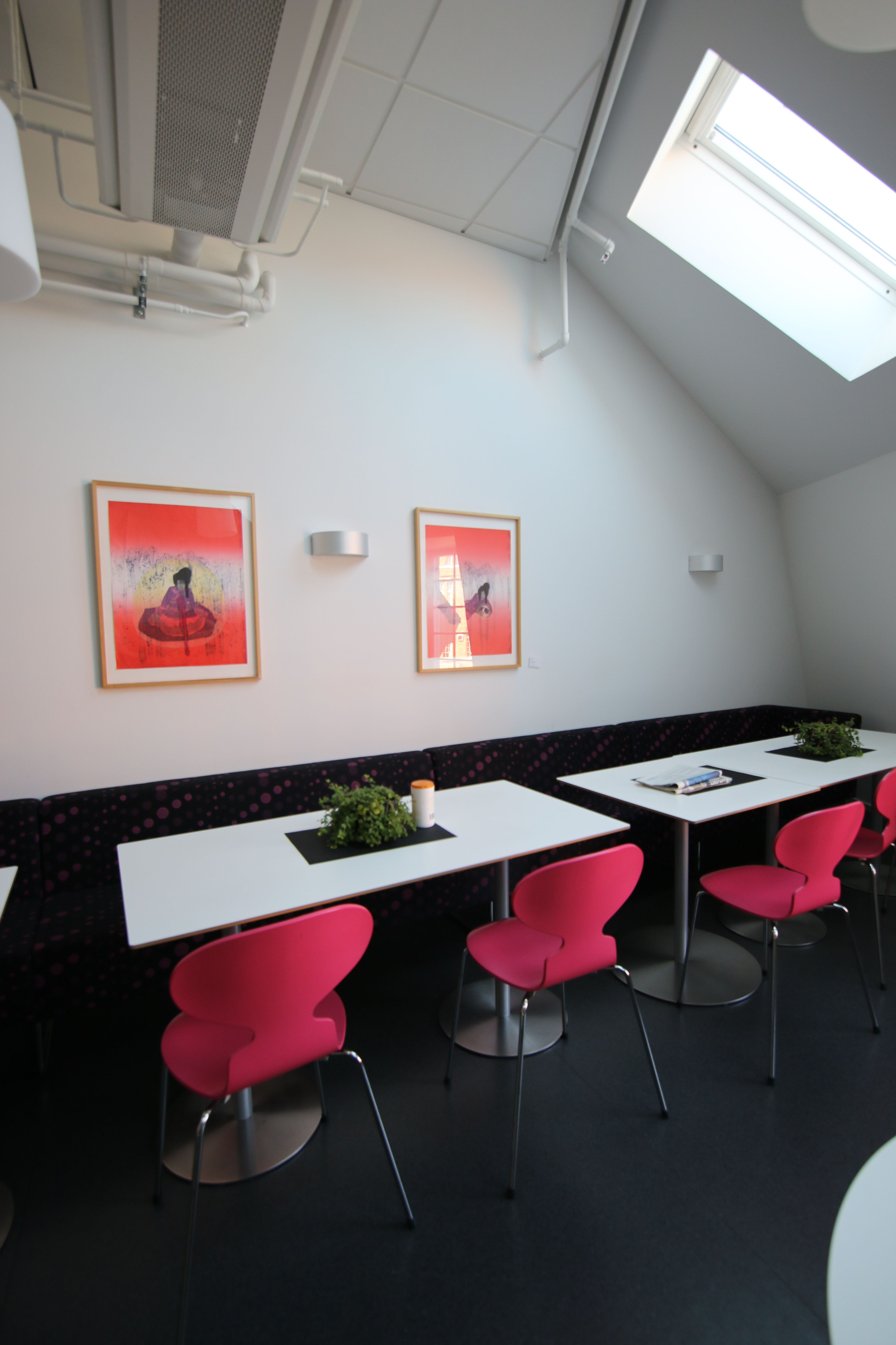
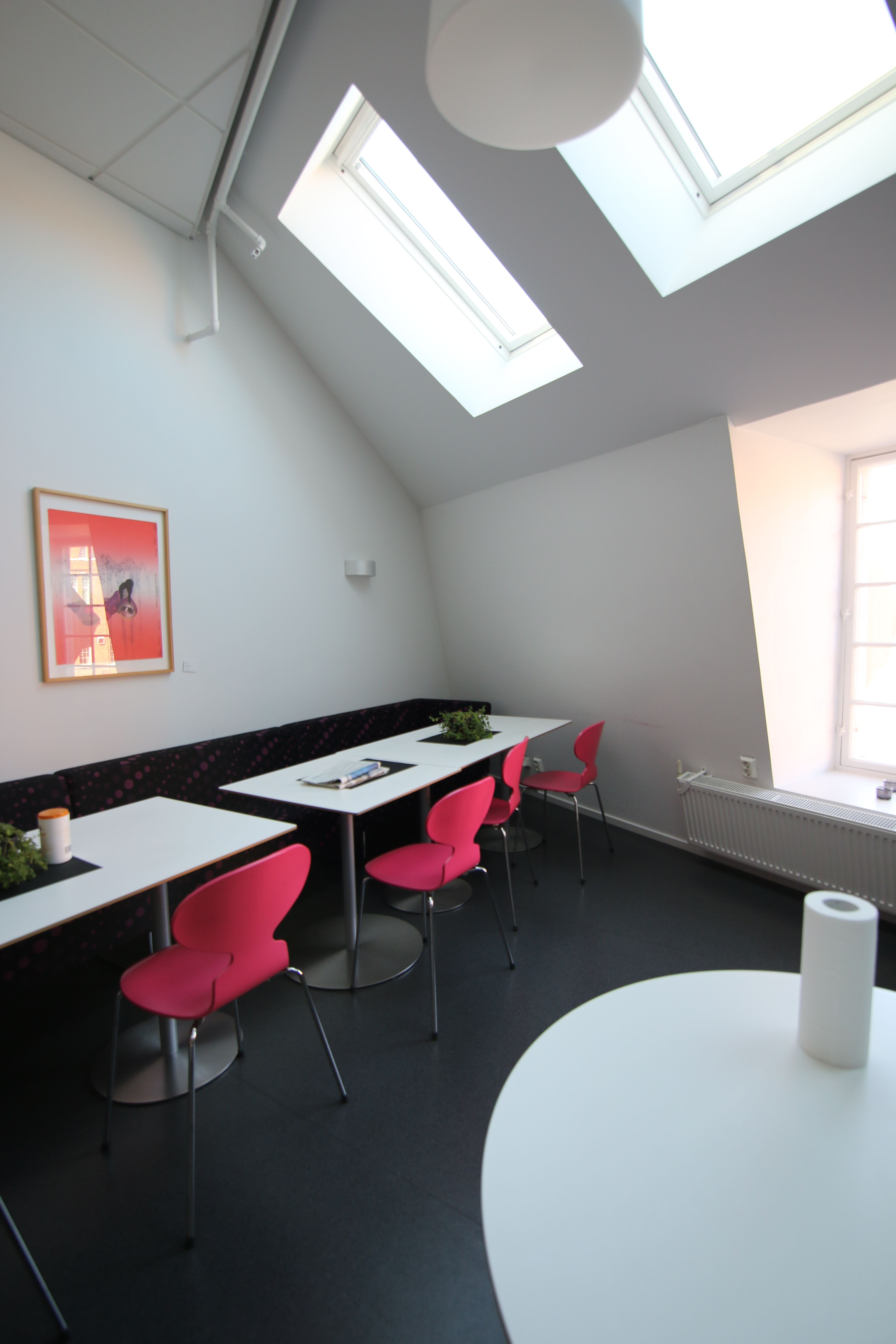
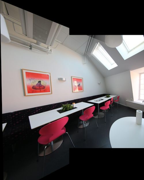
Panoramic Mosaics
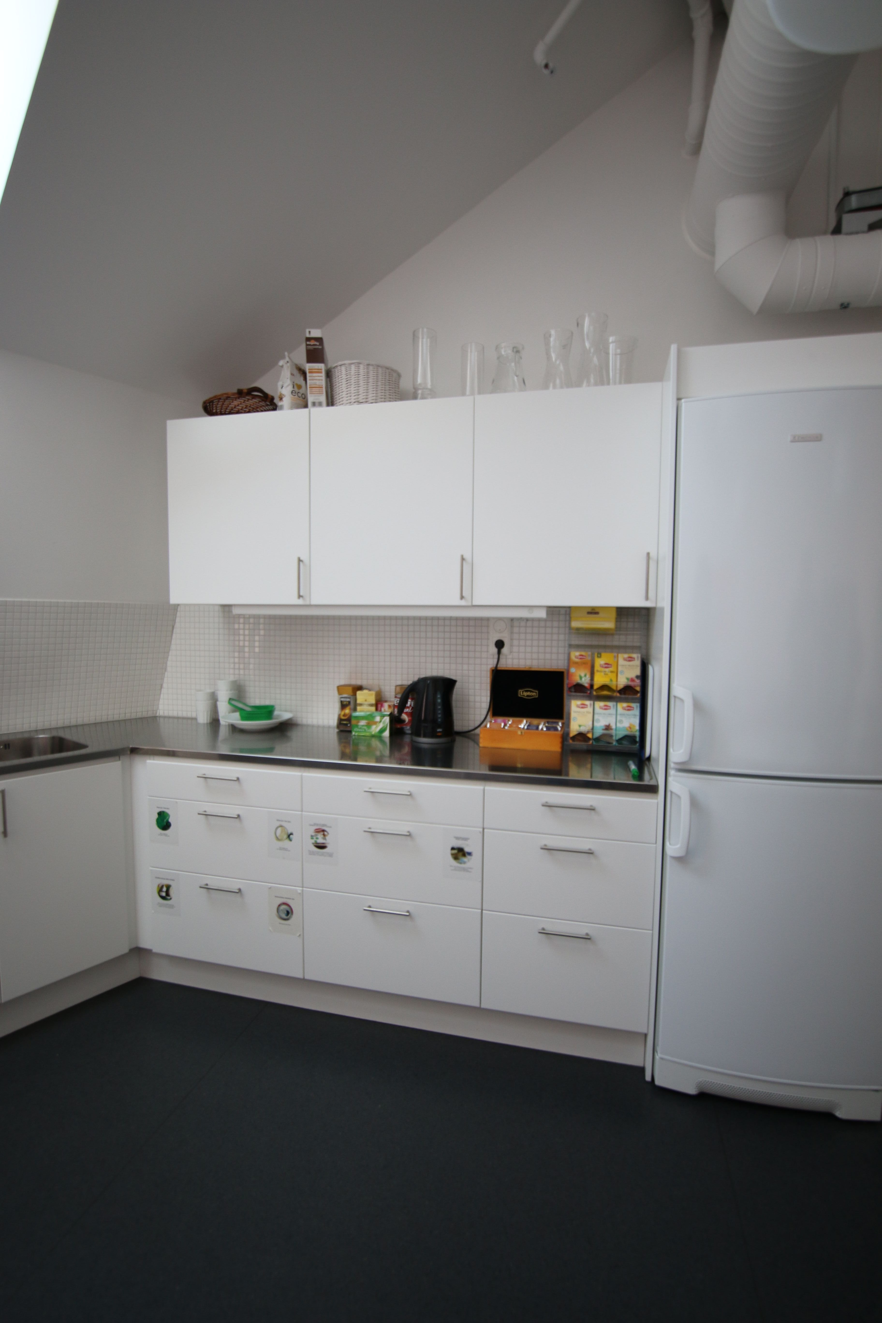
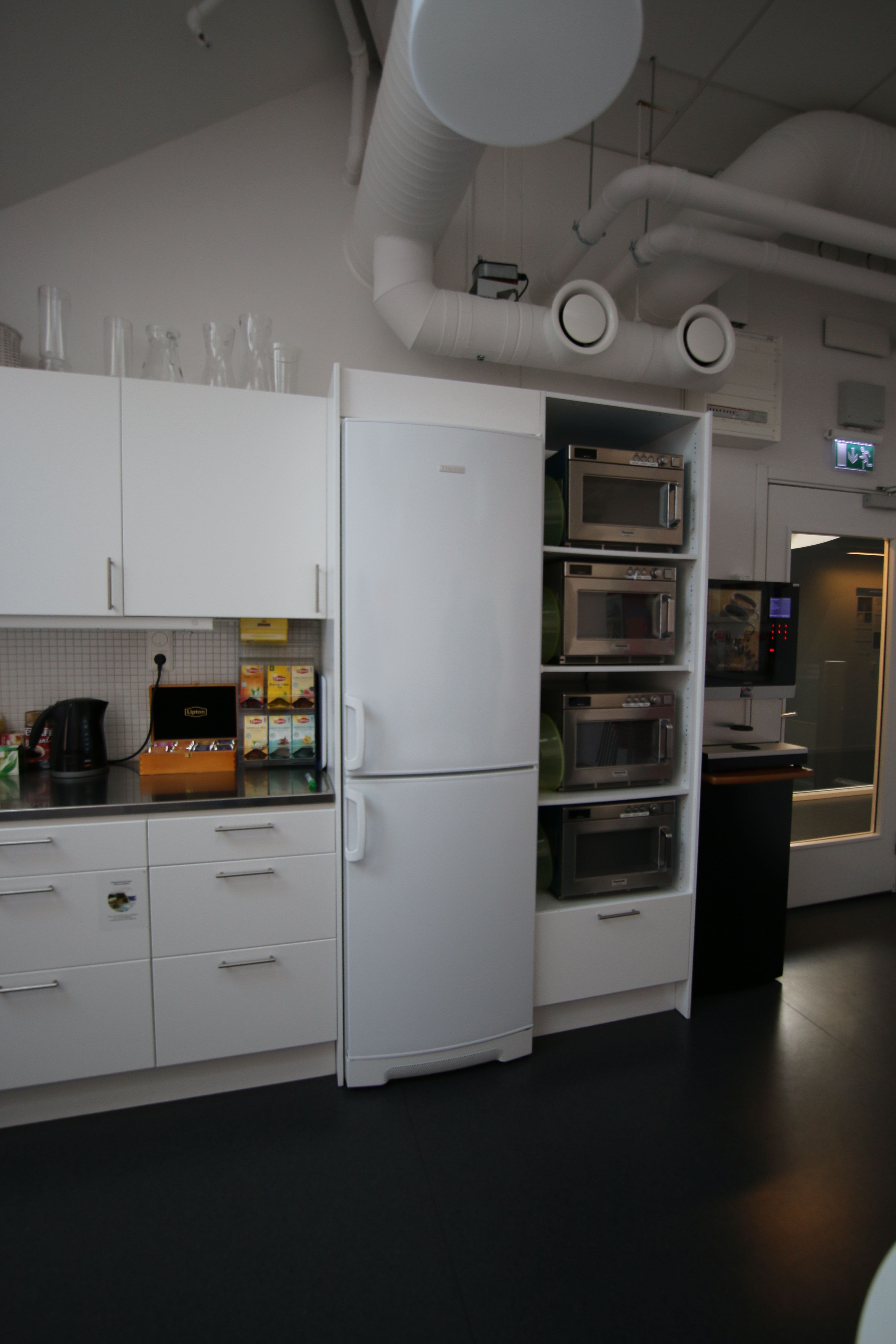
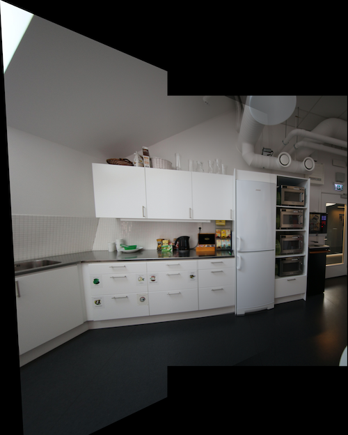
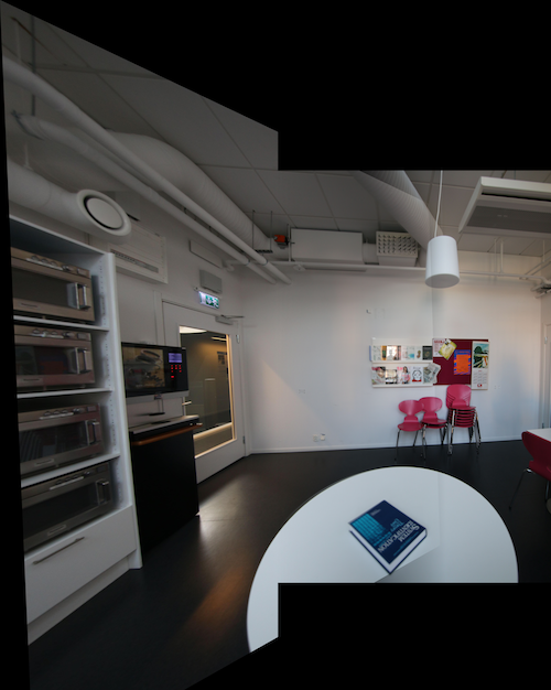
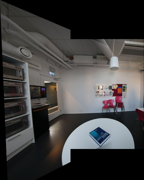
We can create image mosaics by warping multiple photos so they are in the same plane. To warp two photos together, I warped the left photo onto the right photo and then blended them together using linear blending.
To blend, I simply took the weighted average of each overlapping pixel between the two images, where the weight is determined by how far each pixel is from its source. For non-overlapping photos, we can simply copy their original RGB values to the resulting image. Below are some panoramas stitched from images taken from this dataset.


Part B: Feature Matching for Autostitching
In part A, we manually selected correspondence points between two images, then computed the projective transform matrix from these points to warp one image to the space of another image and blend the two images in a mosaic. In this part, we will follow the steps outlined in Multi-Image Matching using Multi-Scale Oriented Patches by Brown, Szeliski, and Winder to automatically determine correspondence points between images.
Feature Detection
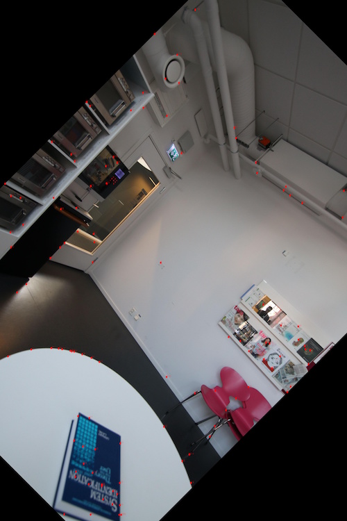
First, we detect corner points in an image by using an algorithm to determine Harris points. A Harris point is determined by locating a point in the image with a large spatial gradient in all directions. If we run the Harris points algorithm using the provided harris.py file, we get an enormous number of points (around 300k points). So, we can filter out some of these points by changing the min_distance parameter in the peak_local_max, which specifies the minimum distance each point should be from another point, or by simply selecting the 5000 Harris points with the highest h-values using the num_peaks parameter. Some Harris points of an image I used to stitch together a mosaic are displayed below.
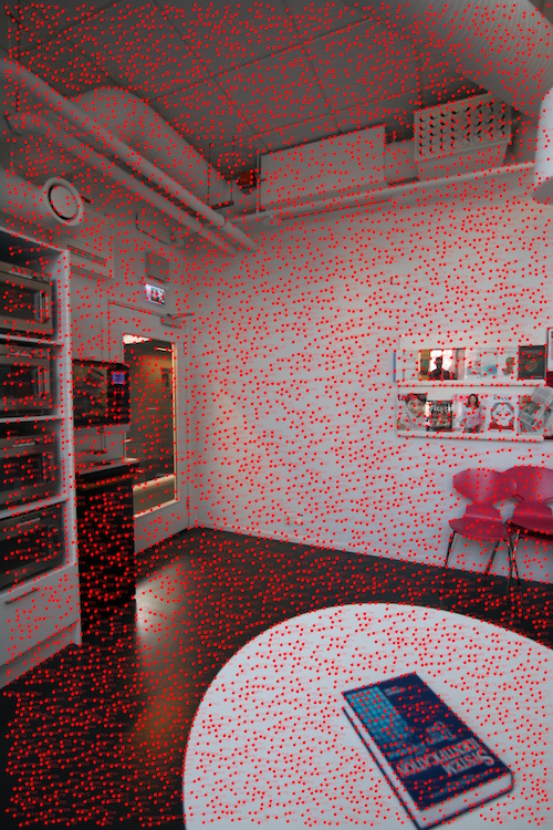
min_distance of 25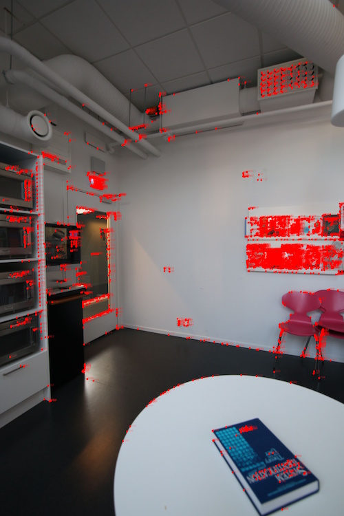
Adaptive Non-Maximal Suppression
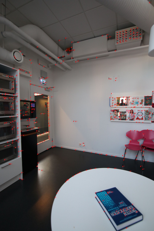
Since the Harris algorithm yields an enormous number of points, and selecting the top n points with the highest h-values yields very densely clustered points, we want to find a way to cut down on the number of points while keeping the points evenly-spaced. We can use the Adaptive Non-maximal Suppression algorithm to find an evenly-spaced distribution of points. For each point, we define its radius as its distance to the point that satisfies this criteria:
After computing the radius value of each point, we can sort by descending order to get the 500 points with the highest radius. The result looks like this:
Feature Descriptor Matching
Now that we have a reasonable number of points, we need to find a good feature descriptor for each of the points so we can match them and develop a point correspondence between two images. For this part, I used Multi-Scale Oriented patches, which is a descriptor that is invariant to scaling and rotation. I considered a 40x40 patch surrounding a point, then downsampled it to an 8x8 patch. Then I normalized the patch by subtracting the mean and dividing it by the standard deviation.
After extracting feature descriptors from each point, we can match corresponding features in each image by looking at the ratios of a feature's distances to its 1st nearest neighbor and its 2nd nearest neighbor. If the ratio is below a certain threshold, then we can call it a well-matched pair. Below are some corresponding points that were computed using this method.

Random Sample Consensus (RANSAC)
Now that we have the point correspondences from feature matching, we must get rid of any potential outliers in the correspondence. We can use the RANSAC algorithm to determine which points are truly inliers. The algorithm is as follows:
- Randomly select 4 pairs of corresponding points.
- Calculate the homography matrix H using these points.
- Calculate the inliers using H. Inliers are calculated as points where $SSD(p', Hp) < \epsilon$.
- Keep track of the largest set of inliers. Repeat steps 1-4.
After finding the largest set of inliers, we use these inliers to recompute the homography and use that as our final homography matrix H. We can then proceed to stitch our photos together using the same methods as part A.
Autostitched Mosaics
Here are some results of the stitched mosaics below, comparing manually selected feature points with automatically selected feature points.


Lessons Learned
Overall, this project was a fun way to explore just how powerful homographies and projective transforms can be. It was also really interesting to see how we can automatically detect features using simple methods like SSD.
Bells and Whistles
Rotational Invariance
I also implemented rotational invariance for the feature descriptors. To maintain rotational invariance, I computed the gradient at each feature point in the x and y directions, and then rotated the window around by the negative arctangent of the y-gradient divided by the x-gradient. Then I simply cropped out the central 40x40 patch of the rotated window, and then performed the normal resizing and normalization operations on the resulting window to get a descriptor vector.
Here are some resulting feature descriptors, and as we can see, they are invariant to rotation.