CS194-26 Project 6: IMAGE WARPING and MOSAICING

Ian Lee

Part A

In this project, we warp an image and stich it with another to create an image mosaic

Homographies

We can recover the parameters of the transformation via a set of (p’,p) pairs of corresponding points taken from the two images. where im1_pts and im2_pts are n-by-2 matrices holding the (x,y) locations of n point correspondences from the two images and H is the recovered 3x3 homography matrix. In order to compute the entries in the matrix H, we can set up a linear system of n equations. Since n =4, we can use four equations to solve for matrix H, however, we will use more points and least squares for a more stable homography recovery. (formula taken from previous year's submissions)

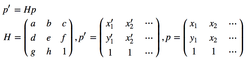
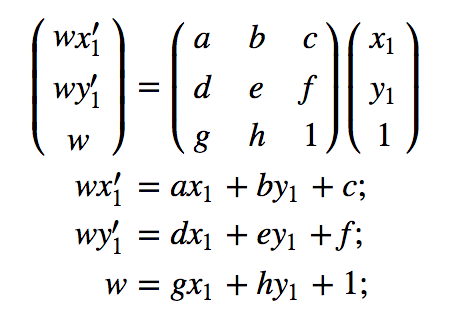
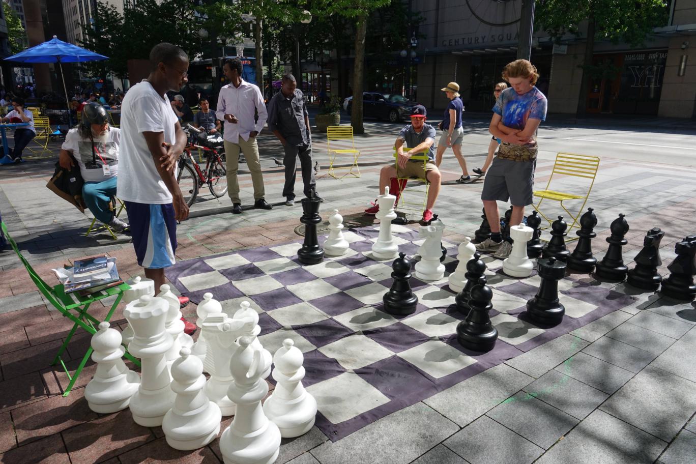
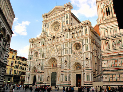
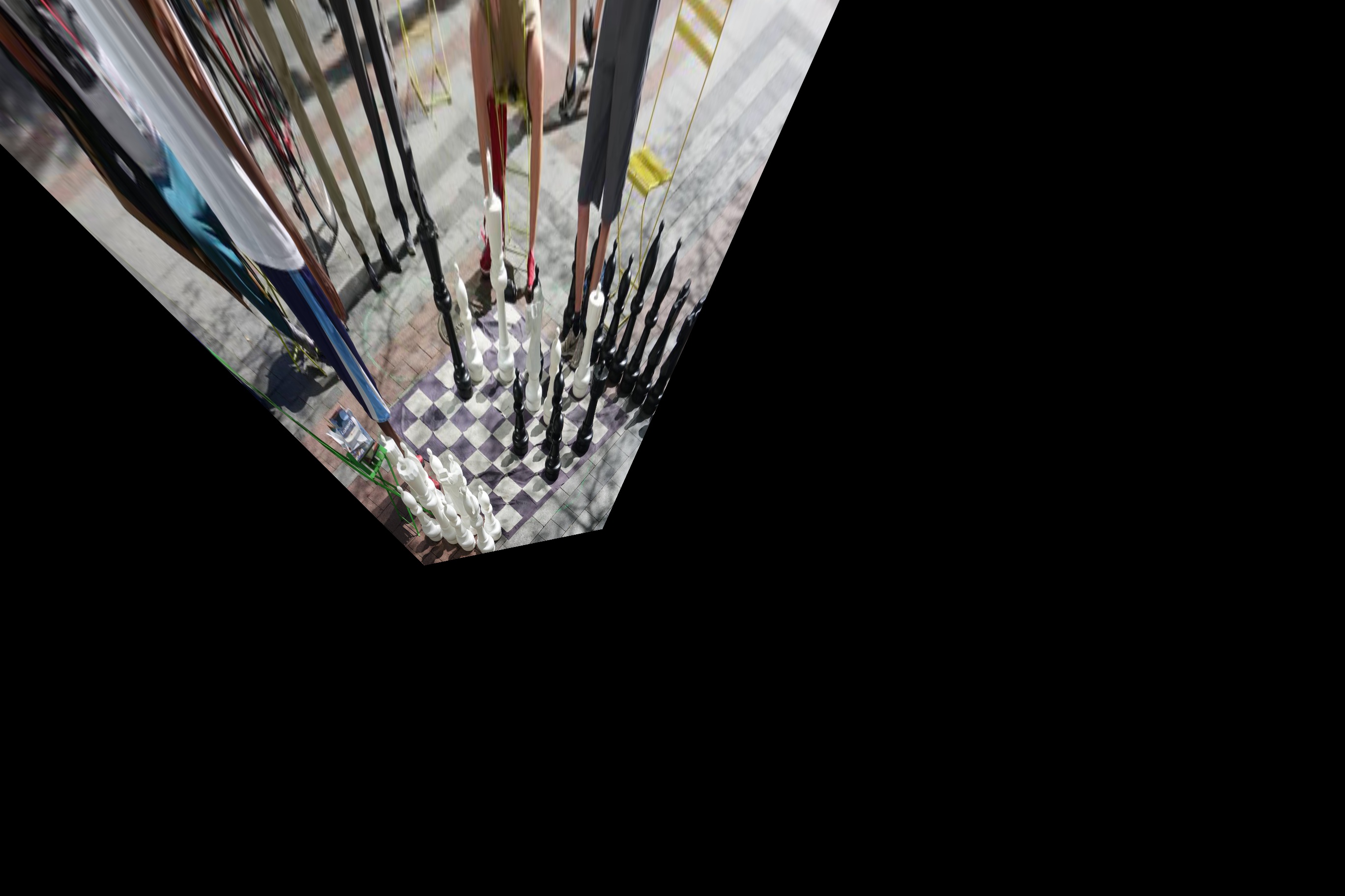
Image Rectification

With our image warping H, we can rectify an image. If we know something in the photo is a square, we can compute the transformation from the four corners to a manually set of four points that define a square. Then we can warp the entire image using the transformation for a rectified image

Chess @ Seattle DT	Florence
Rectified Chess	Rectified Florence

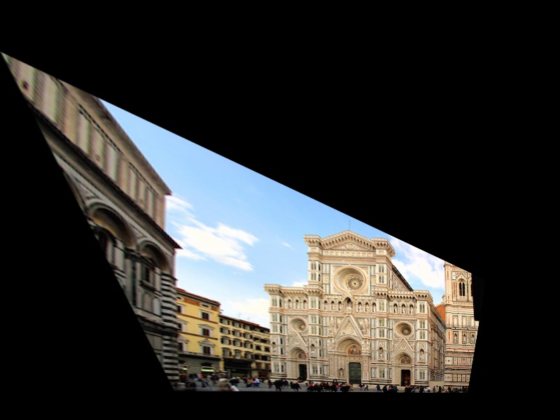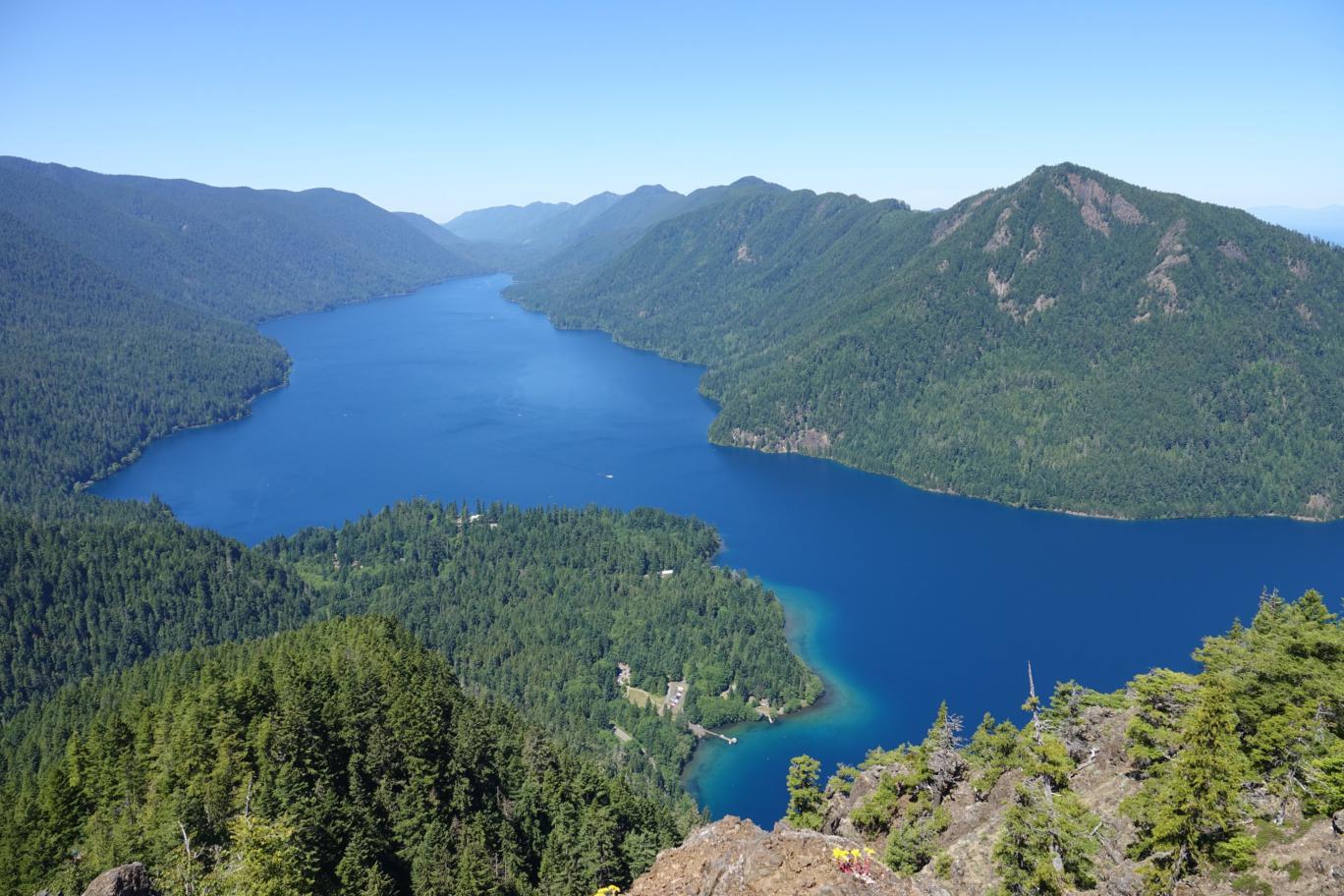
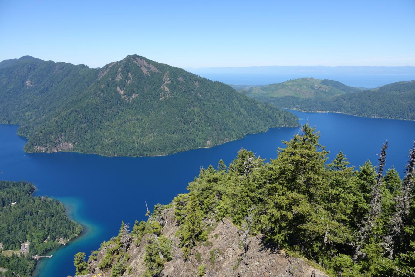
Image blending

with our image warping technique, we can warp images. However the edges of the two images could be obvious if we do a simple weighted average blending. Instead we could use the linear blending technique with an alpha that falls of until it hits 0 at the edges of the unwarped image.

Olympics Park

Average Blending
Feathering Averaging

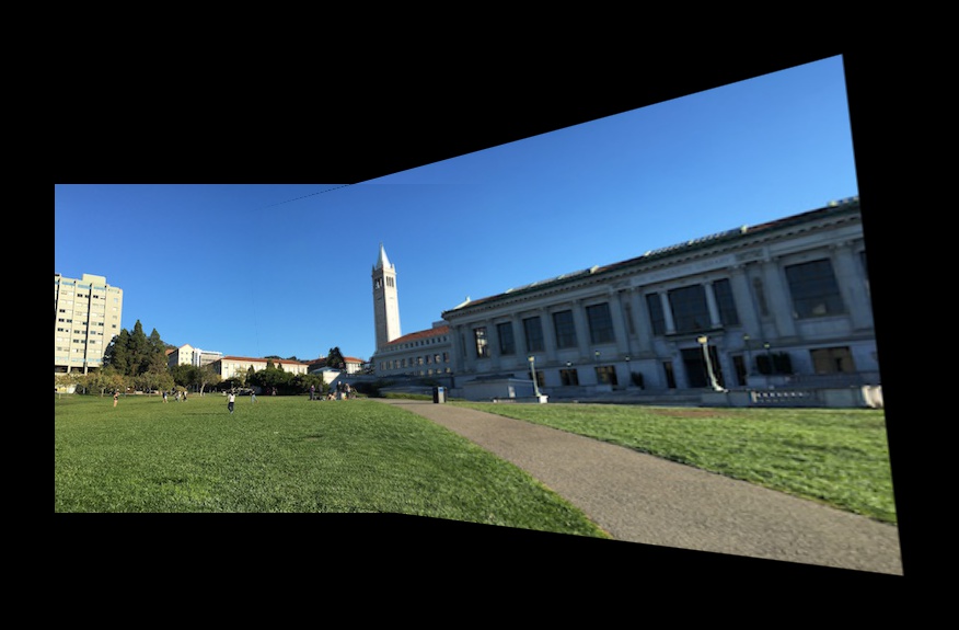
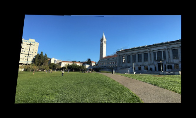
Berkeley1	Berkeley2

Feathering Averaging

What I learned

The project is really cool as I learned how panoramas are made. With the techniques that I learned, there are so many ideas that I could think of, unfortunately, I don't have time to implement some Bells and Whistles this time.

Part B

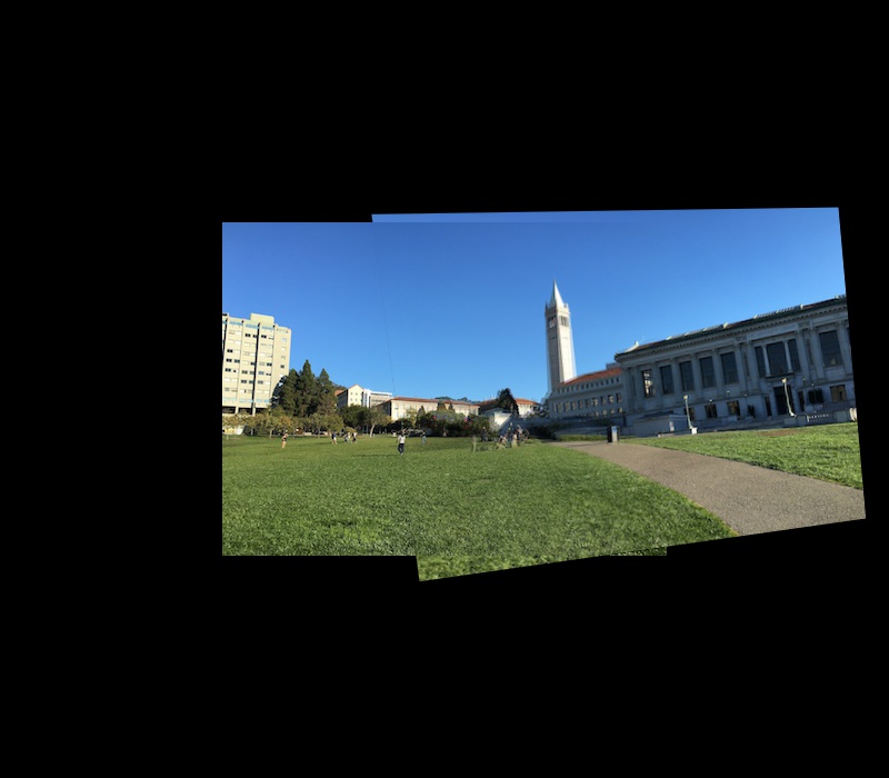
In part B, I attempted to implement autostitching, instead of having to pick the points by hand, I followed the paper “Multi-Image Matching using Multi-Scale Oriented Patches” by Brown et al to automatically identify correpondence points in two images

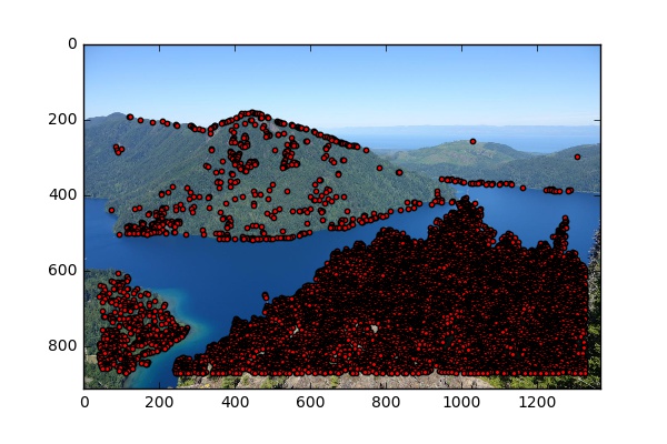
Step 1: Harris Interest Point Detector

We want to find the corners in the image. Supposed we have a viewing window, if we are looking at a flat surface or an edge, we should be able to move our viewing windows without seeing significant change. Therefore, we are only interested in "corners", which are the points that can be more easily matched between two images. With the Harris Corner function provided, we are able to retrieve the corner strengths of every pixel in the image. Here I will show the pixels with corner strengths/ max(corner strengs) > 0.05

Image1 strenths	Image2 strenths
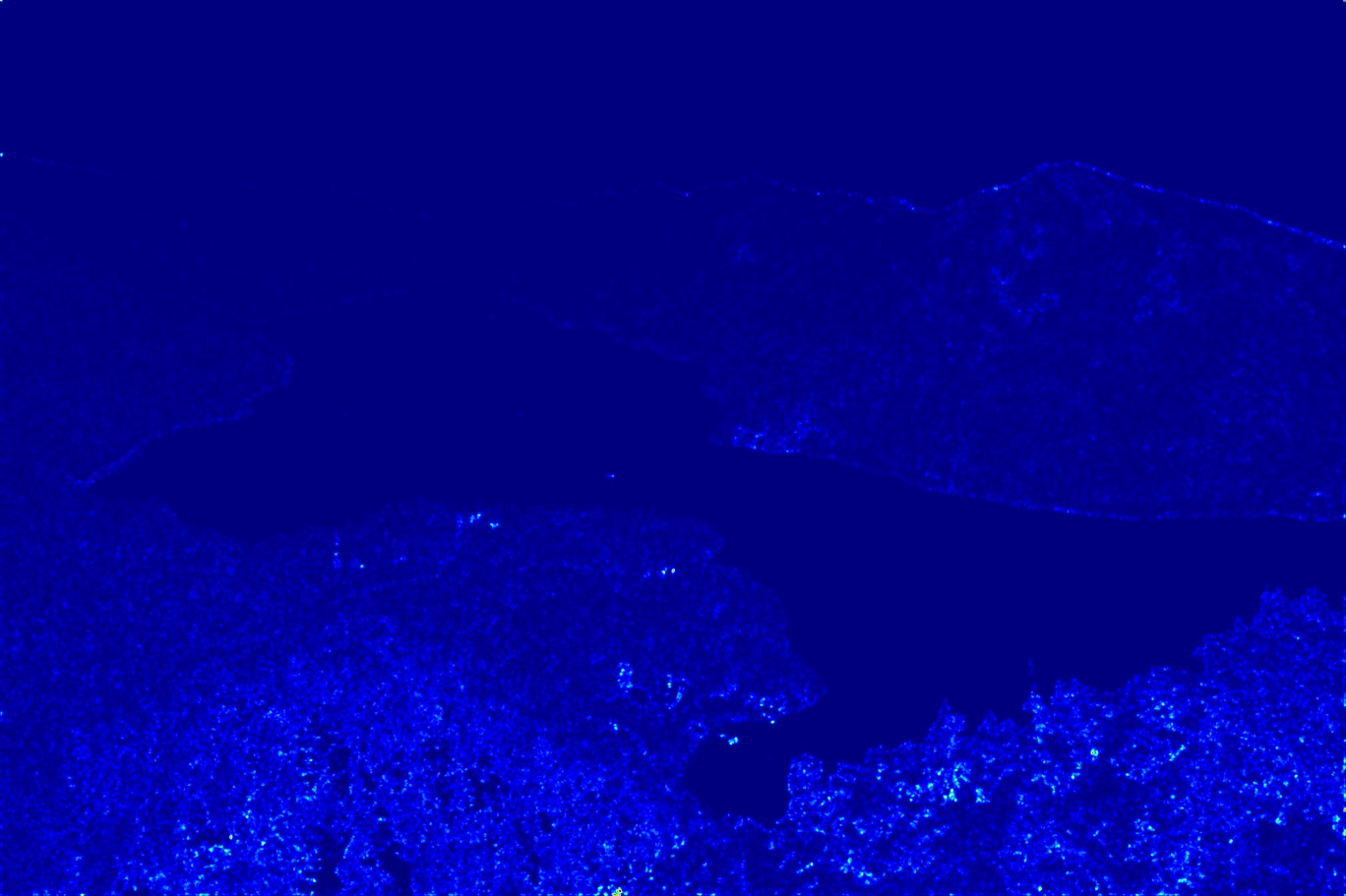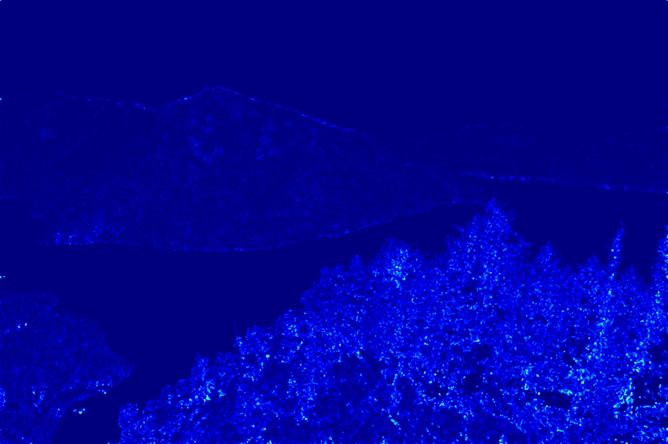Image1 harris corners	Image2 harris corners

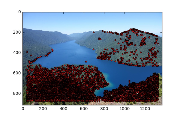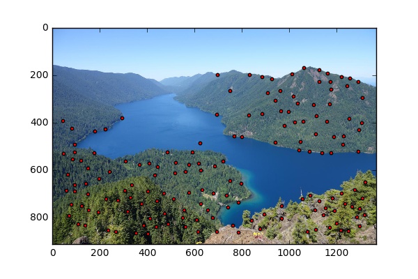
Step 2: Adaptive Non-Maximal Suppresion

We see that there are a lot of points and we would want to take the top performers. However, if we simply increase the threshold, we might end up with a lot of points clustered around an area. It would be disastrous if the overlap area does not contain any of those points. Therefore, we want to select the top performers but also keep in mind of their distances from one another. To do so, we can calculate the anms value for each interest points, which is the largest radius in which the interest point is the strongest. Then we pick the top 200 points with the largest radii.

Image1 ANMS	Image2 ANMS

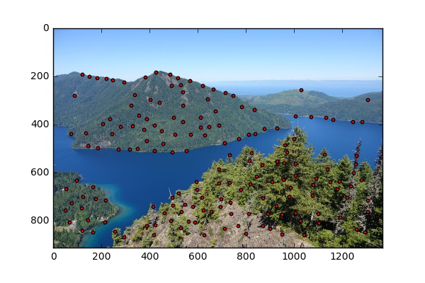Step 3: Feature Descriptor

Now with our trimmed list of interest points. we would want to find correspondences between the two images. To do so, we would want to extract features from each point. I took a 40*40 patch centered at each interest point and downsampled it to 8*8. I also adjusted each patch to have zero mean and a standard deviation of 1, which makes our patches invariant to lighting.

Step 4: Features matching

We can use l-2 distance to compare patches. However, we would want to introduce a new trick The Russian Granny Algorithm at this step. We want to find the best match and the second best match for each patch. We only call it a match if the best match is significant better than the second match. Here I used a ratio of 0.4.

Image1 Features	Image2 Features

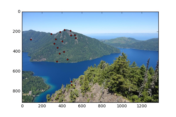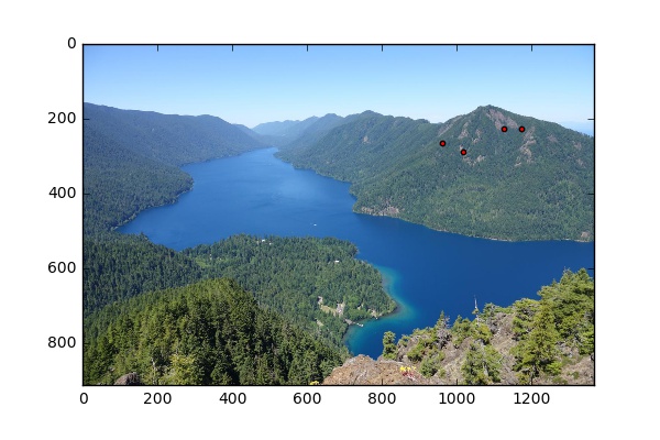
Step 5: Ransac

Finally, I used ransac to choose the 4 pair of correspondeces for computing the homography matrix. I picked 4 pairs of correpondences, computed the homography, performed homography on all matches, and summed the errors, for 5000 times. Then I picked the homography and the set of points that have the smallest error.

Image1 Optimal features	Image2 Optimal features

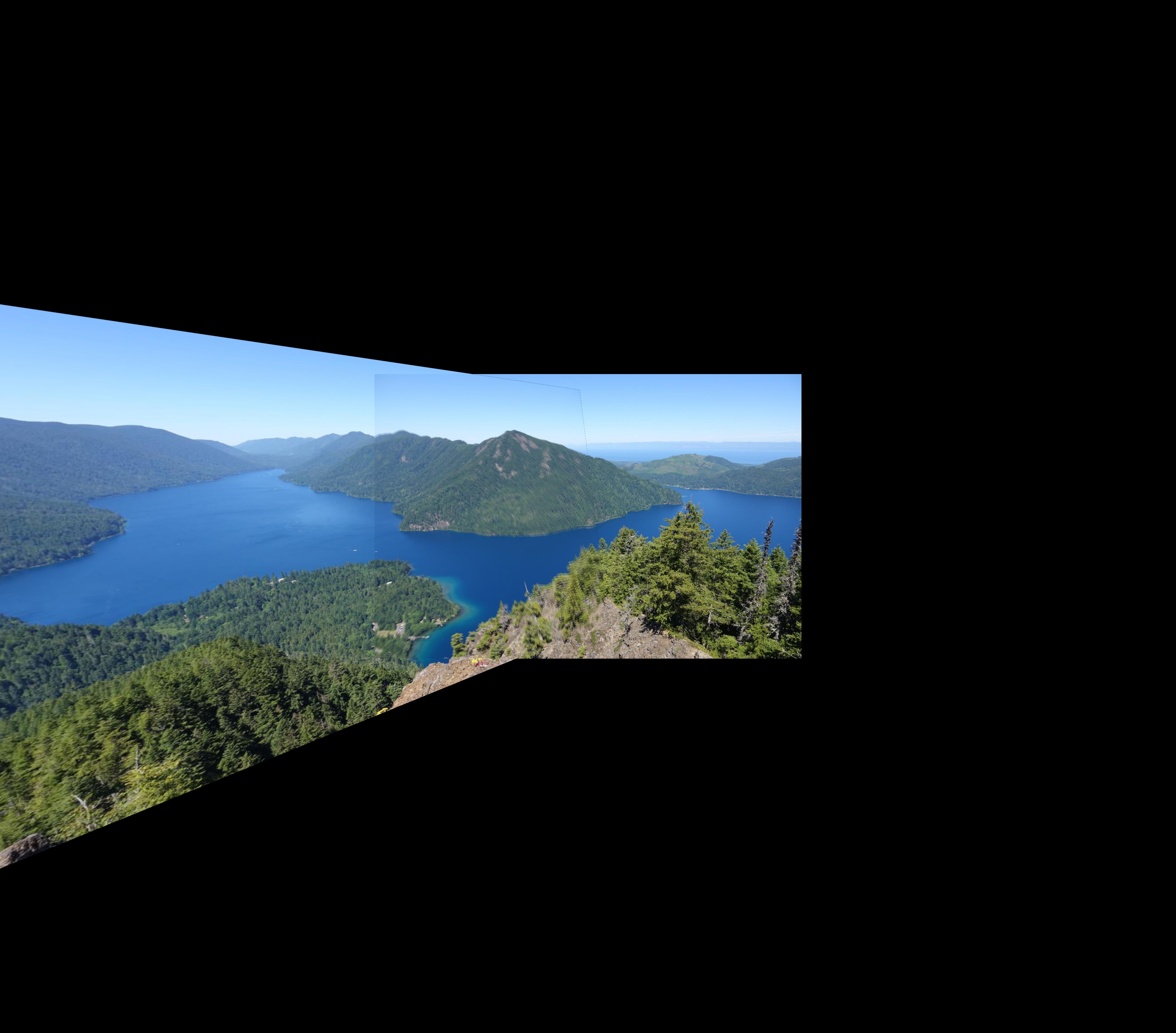
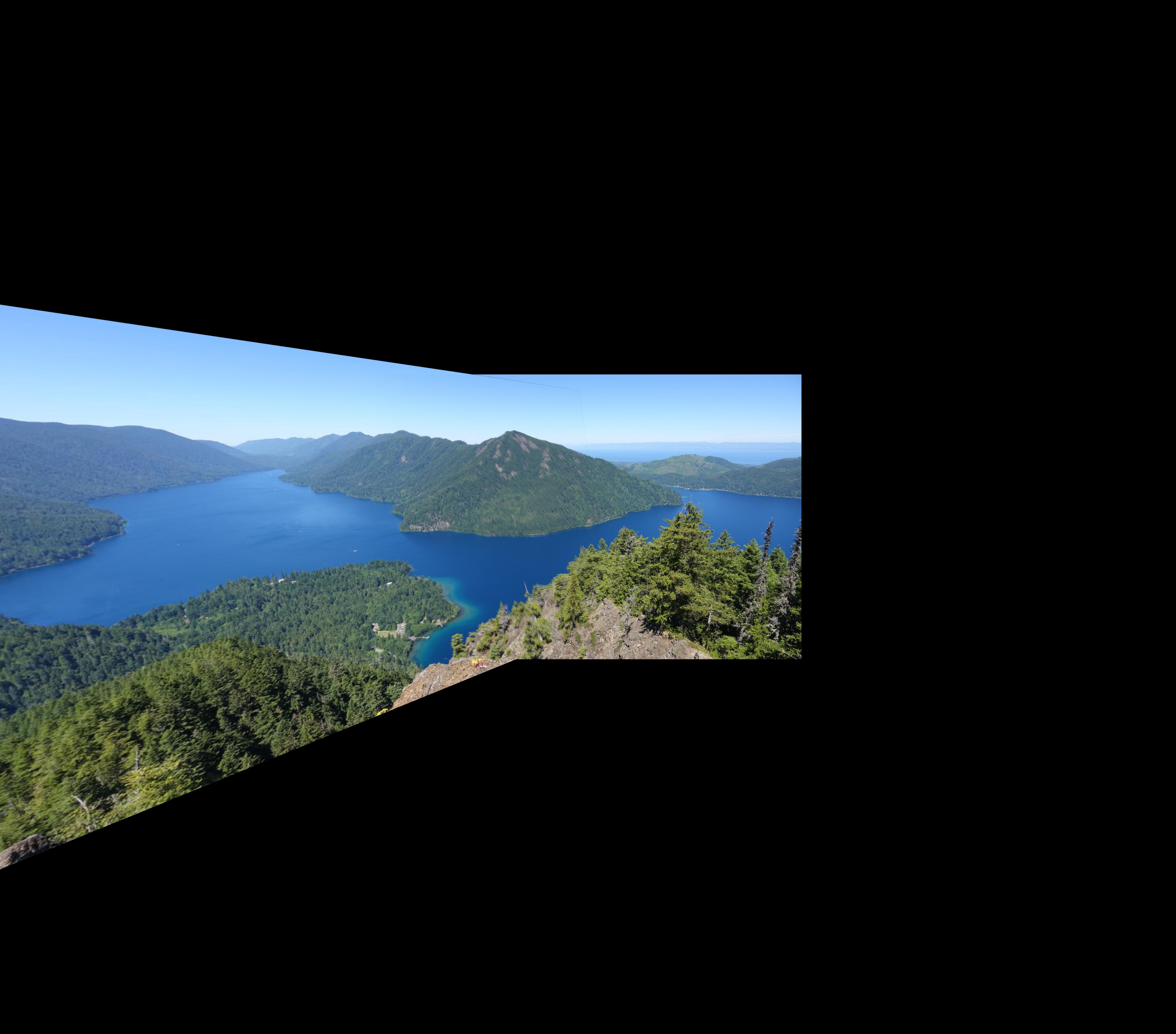
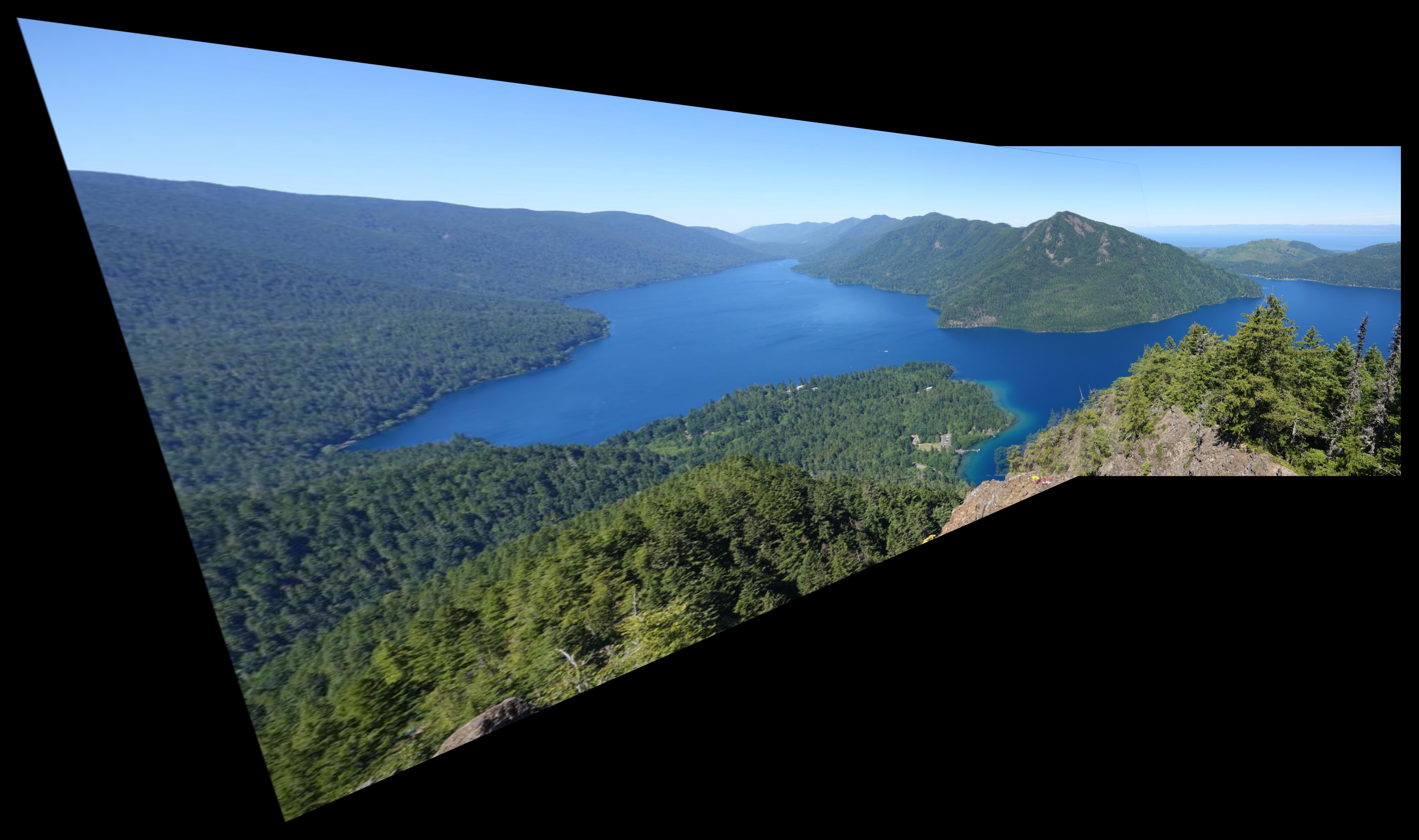
Olympic autostitching

More photos

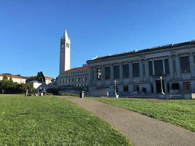
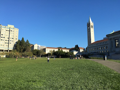
Berkeley left	Berkeley right

Me in Vancouver
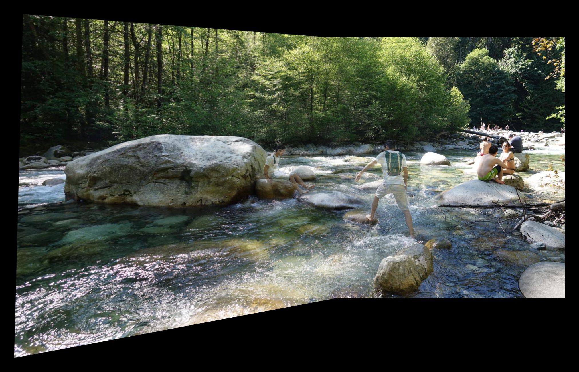Sydney
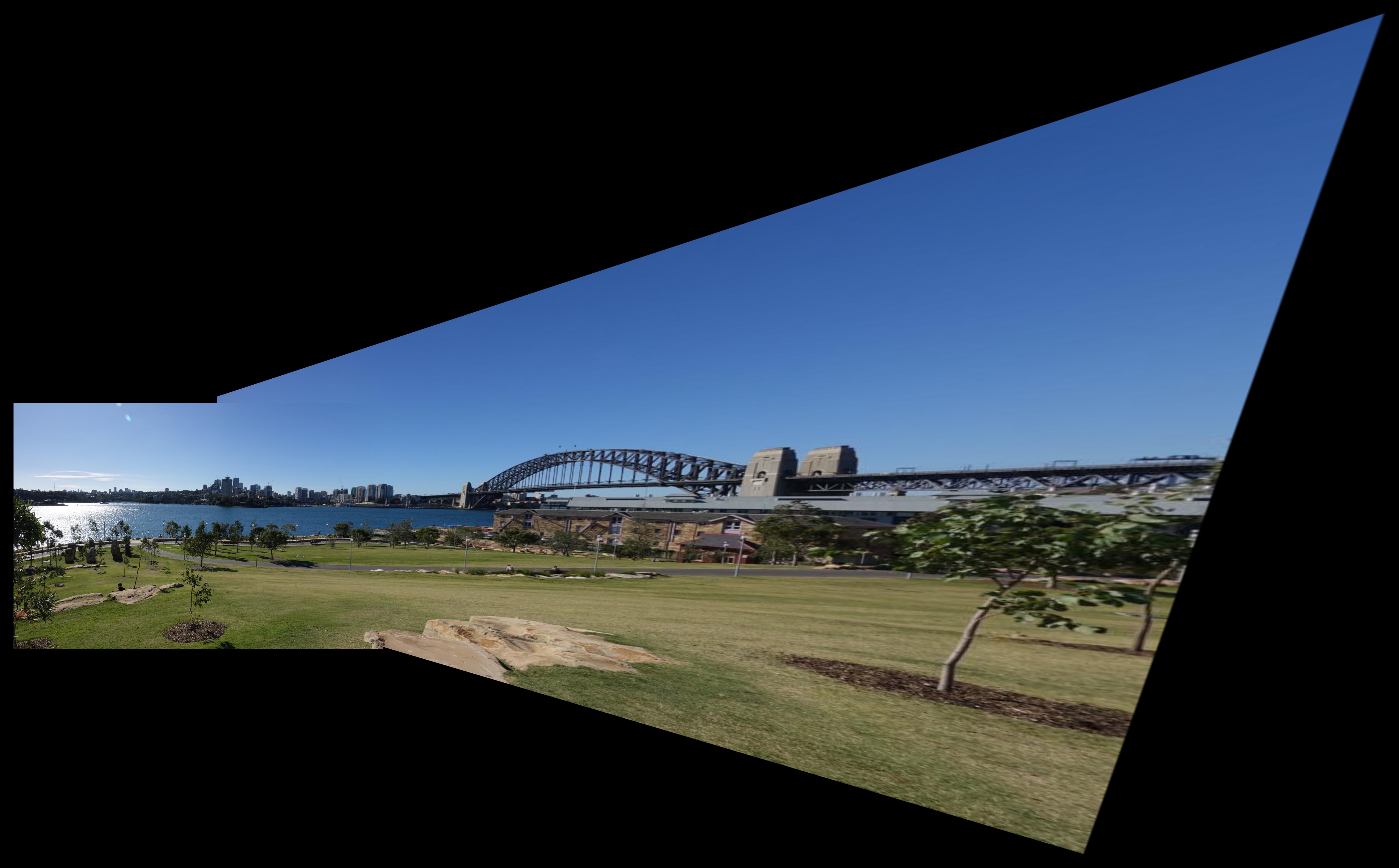Duck in Vancouver

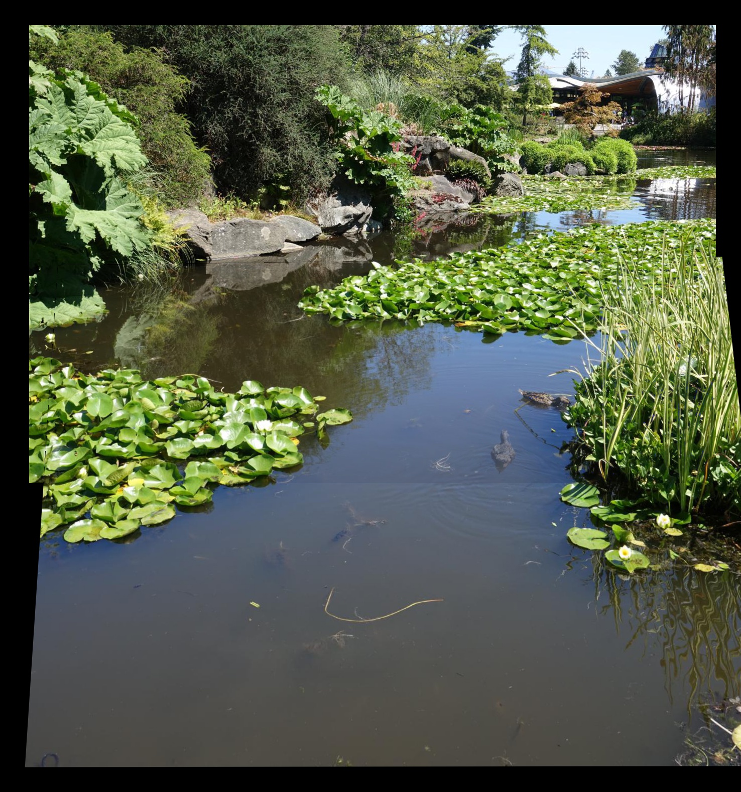What I learned

In this part, I learned two great tricks that have lots of applications in the Russian Granny Algorithm and Ransac. The code also makes stitching images a lot easier with autostitching