Project 6A: Image Warping and Mosaicing

Part 1: Shoot and Digitize Images

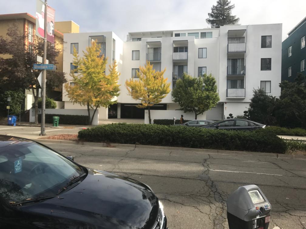
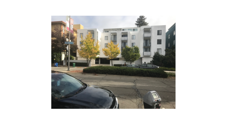
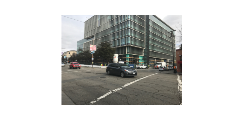
When taking pictures of a scene, it's important that the camera does not leave it's pivot point. The camera is rotated from a single point, in which the images of the mosaic have 40-70% overlap. This will be important when we define our correspondences between the two images. Here are the pictures I took with my iPhone 7 camera. Unfortunately iPhone automatically adjusts aperture, so the photos when combined are going to be slightly off in coloration. Additionally, since I do not own a tripod, pivoting my phone centered at the camera was quite challenging. All photos were taking near North Berkeley.

Part 2: Recover Homographies

Overview: in order to merge two images into one we first must warp one image into the plane of another. To do this, we must recover the homography that warps between the two images. A homography is a linear transformation, H such that p' = Hp, where p and p' are homogeneous coordinates of the 2 images.

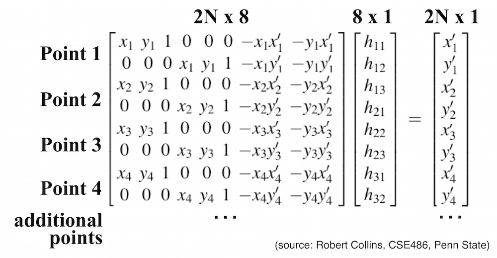
So H is a 3x3 matrix, but we set the 9th entry to 1, so we have 8 degrees of freedom/variables we want to solve for. Computing the exact H is an overconstrained problem, so we approximate H using least squares by solving the equation Ah=b. In order to compute the homography matrix I constructed the following optimization problem.

Part 3: Warp the Images

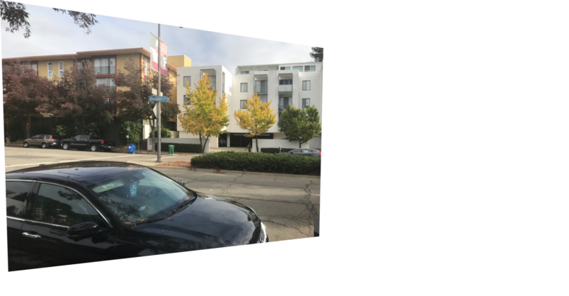
Overview: this part was considerably trickier. I used the same logic of warping from project 4, except this time we were allowed to use library functions. In order to calculate the shape and the size of the output image in such a way that the whole warped image fits onto the canvas I piped the corners first and created a new transformation matrix to dot it with the original homography matrix so that it also takes care of shifting the warped image by the necessary offests. Using the max and min values of x and y for the piped corners I also found the new output shape to pass into the skimage transformation warp function.

Image Rectification

Overview: At this point in order to make sure both the homography calculation and the warp function behave properly I attempted to rectify a number of images with items that have a square like objects with planar surfaces. I rectified by warping the images so that that plane is frontal-parallel. The original points were chosen manually, and the new points were chosen manually as well, through guess and check to ensure the correct width to height ratios were used. Top three examples are of pitcures I took myself and the last one is a photo I found on the Internet.

Frontal-parallel plane - keyboard.

Frontal-parallel plane - mirror.

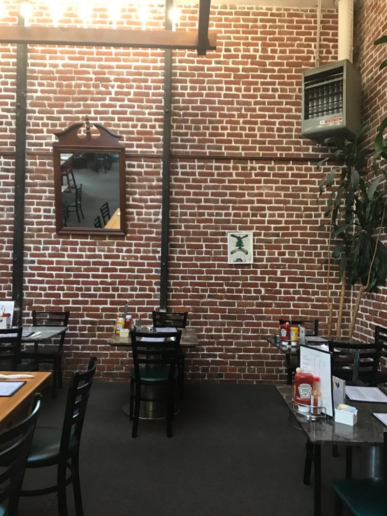
Frontal-parallel plane - heater in the corner. Image was cropped to see the heater better.

Frontal-parallel plane - canvas with the hot air balloon.

Part 4: Blend the Images into a Mosaic

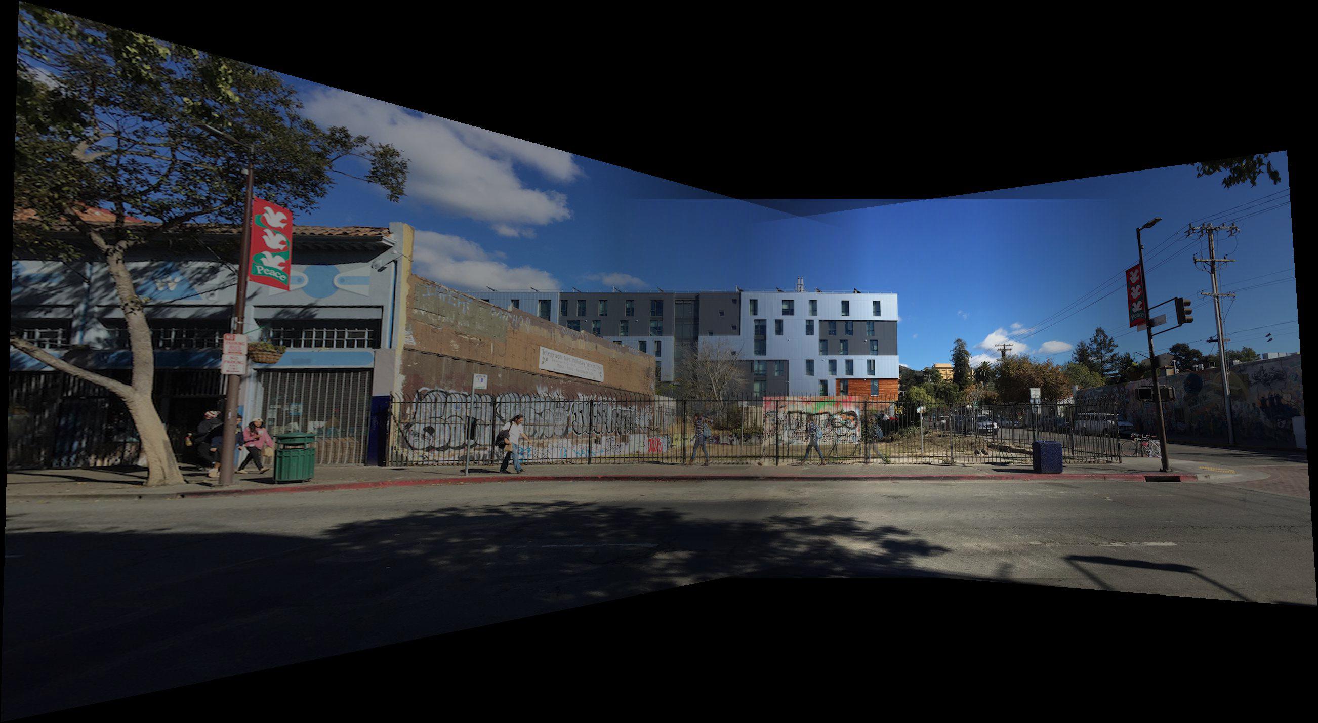
Overview: all of the previous steps have been leading to this most challenging part. For all panoramas I shot three images and calculated the homographies of the right and the left images into the plane of the center (middle) image. Before warping images I added an alpha channel to each one in order to do simple weighted averaging later. I proceeded to calculate the output size of the entire panorama and the offests (added to original homographies) for all three images. I then warped each image using the appropriate homography and output shape. Then to combine all three images I simply extracted the alpha channels of each three warped images and added them together. This allowed to to identify where certain pixels had overlapping values from multiple images. Then I averaged those pixels by dividing the summed image (of all three warped images without the alpha channel) by the sum of alpha channels. I've provided three uncropped examples below.

You will notice that the first two examples are slightly blurry. This is because the manually picked correspondence points are not very reliable. Furthermore, the images were taken from approximately the same point but not exact.

I also played around with another blending techinque described on the website. I set the alpha in the middle of an image to 1 and slowly trickled down to 0 off to the sides. Below is an example of such blending based off of images I borrowed from a friend.

Part 5: Lessons Learned

I learned that warping has some very powerful applications and that correspondece points play a big role in precision. It was nice to play around with linear algebra and figure out why certain things were not working as expected because there was always a logical explanation that could be calculated.

Part 1B: Harris Interest Point Detector

This is the beginning of the second part of the project, where we attempt to automatically find features to match our images on. Harris corner detection algorithm will help us with that. We were allowed to use code provided by the GSI so I played around with some sigma values (ultimately 3 for this image resolution) and here is an example result of a harris corner detection algorithm.

Part 2B: Adaptive Non-maximal Suppression

We implement Adaptive Non-Maximal Suppression because the computational cost of matching is superlinear in the number of interest points, so we attempt to restrict the number of interest points in each image. At the same time we aim for interest points to be distributed evenly across the image, since for image stiching applications the area of overlap might be small. ANMS works by setting a suppression radius at infinity, and gradually decreasing it. A point is suppressed if it is not the strongest corner (as determined by the Harris detector) in the radius. We decrease the radius until a given number of points are not suppressed. In practice, my implementation computes the suppression radius for each point (We use a value crobust = 0.9, which ensures that a neighbour must have significantly higher strength for suppression to take place.) sorts the points by radius, and truncates the list based on the requested number of interest points. The ANMS-filtered harris corners are shown below for the top 500 corners.

Part 3B: Feature Descriptor Extraction

For each feature point, we extract the axis-aligned 8x8 patch in a 40x40 window using a spacing of 5 pixels. We get the 40x40 window around a feature point and downsample it by blurring it and subsampling to avoid aliasing to form a 192x1 vector (with 3 color channels). Then the vector is bias/gain normailzed to give the final descriptor. Here's an example descriptor (non-normalized, non-flattened).

Part 4B: Feature Matching

After extracting feature descriptors for two images that I am trying to align, I attempt to match these collections of features. I calculate a euclidian distance between every pair of features and find the nearest neighboor from the second set of features to each feature in the first set. I also find a second nearest neighbor and compare the ratio between the two distances. This is a good estimator for whether the matched features are actually relevant and not noisy. If the ratio is less than 0.6 I keep the pair as a matched pair.

Part 5B: RANSAC

Lastly I perform automatic stiching on sets of three images by tying all of the above steps together. In the RANSAC algorithm, we randomly select four point correspondances and compute the exact homography. We transform the feature points in the first image to locations in the second image using the homography and count the number of inliers. An inlier is a point correspondance where the location of the transformed point in the first image after applying the homography is within epsilon of the corresponding point in the second image. In other words, the homography does a good job of modelling the relationship between the points in a point correspondance. I set epsilon to be 4 pixels. We find the largest group of inliers and compute the homography matrix using the least-squares approach for better stability. Below you will see comparisons between manually and automatically stiched images.

Single Example

On the left are manually stiched examples, right - RANSAC. You can view the biggest improvement on the last pair of images.

Part 6B: Lessons Learned

I learned that automatic feature detection is very effective at finding a good homography and making beautiful panoramas! Though the automatically detected points are not the same as the points I manually selected, the algorithm still produces a nice panorama.