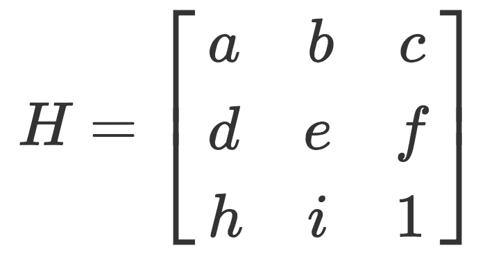
The main idea of this project is computing homographies so we can use them for image rectification and mosaicing. Homographies allow us to take an image and project it to a different perspective. The way we do this is by first collecting pairs of corresponding points (x, y), (x', y') in the original perspective and the desired perspective. This amounts to solving the set of equations:
ax + by + c - gxx' - hyx' = x'
dx + ey + f - gxy' - hyy' = y'
for every pair of corresponding points and where a, b, c, d, e, f, g, h specify the homography matrix:
Notice that this reduces our problem to a least squares problem and we are simply solving for a flattened H.
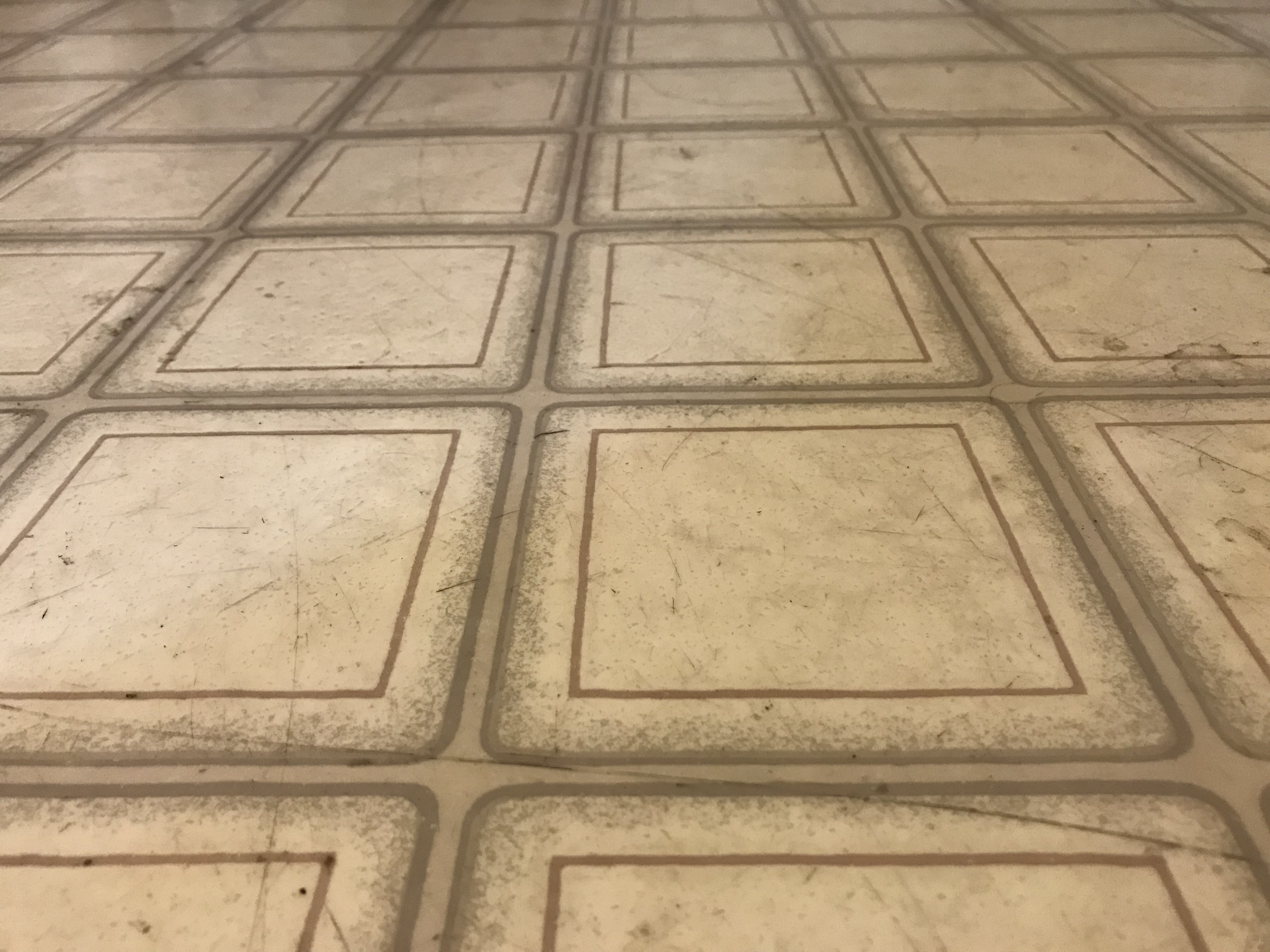
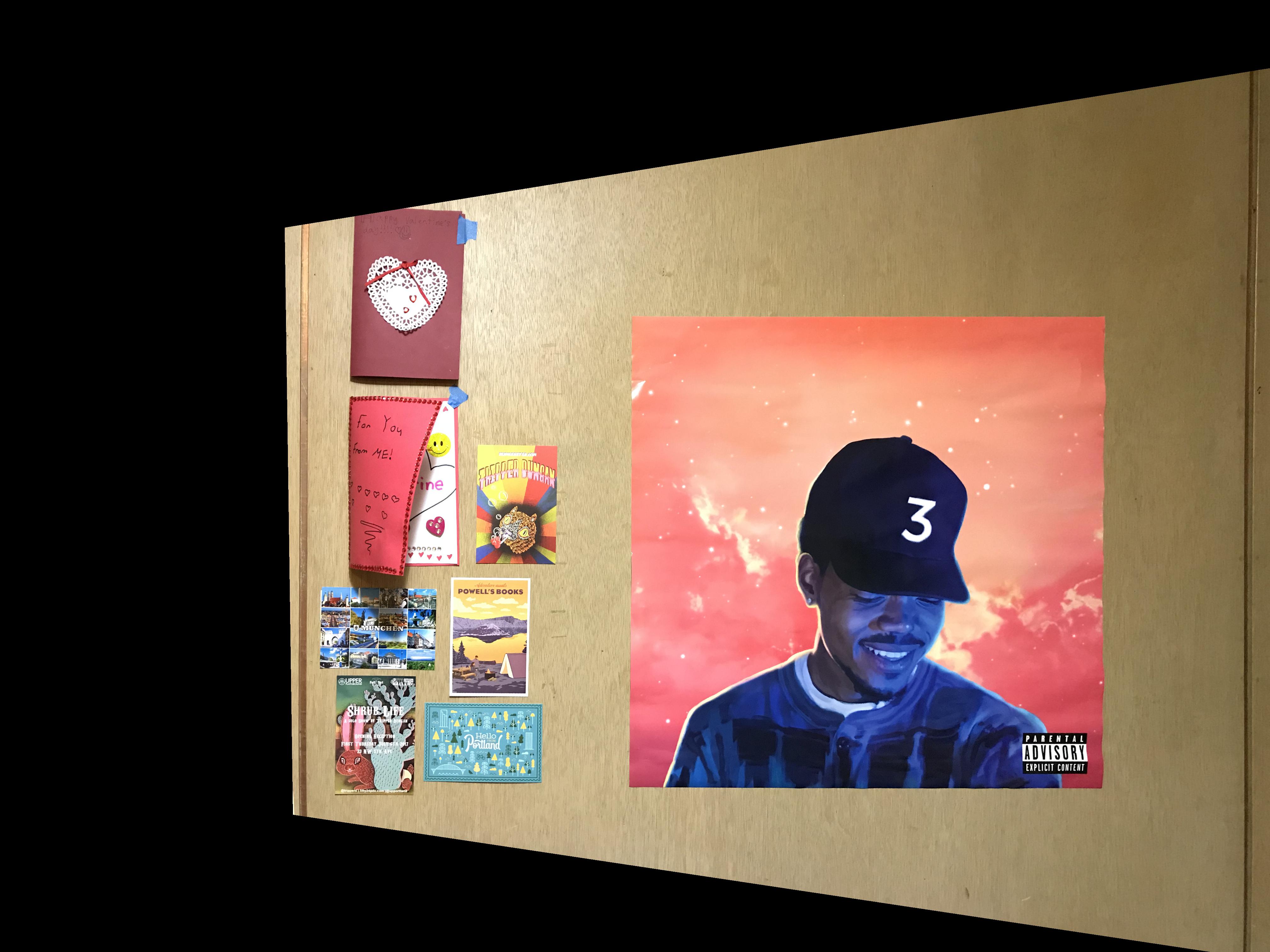
For this part, we took pictures of scenes that had square objects in it but appeared skewed. Then we warped them so they would look square again. We define the correspondence points as the corners of the square object and the points (0, 0), (0, 1), (1, 0), (1, 1) scaled by some number and translated.
 |
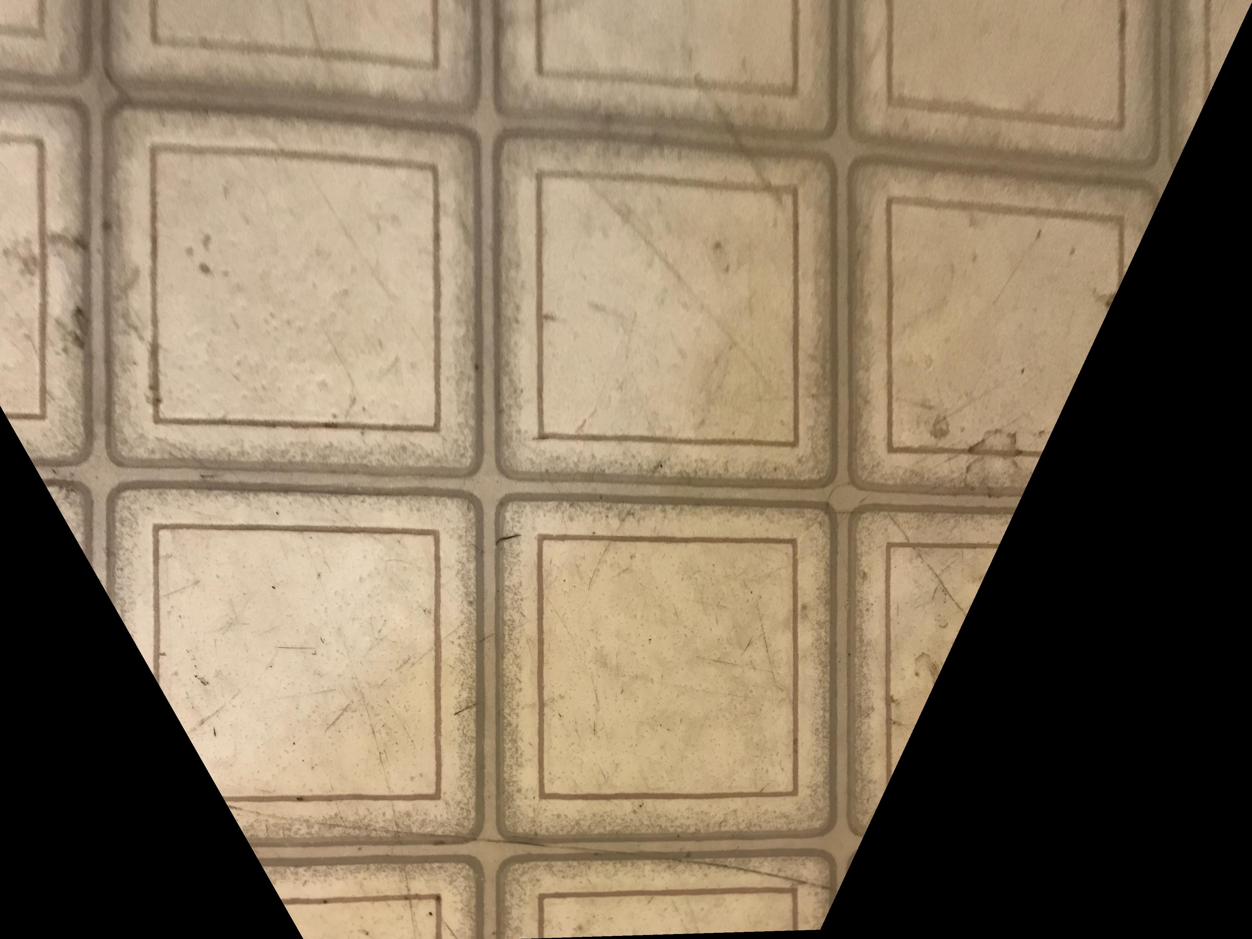 |
| Original image (has square floor tiles) | Rectified image |
 |
 |
| Original image (has square poster) | Rectified image |
For this portion, we do a few things to create a mosaic. First, we take images of a scene with the same optical center. We then recover homographies between the images. Once we've warped the images, we can composite them by doing a simple feathering in the intersection of the images. This feathering is simply a linear falloff in the intersection region of the masks of the images.
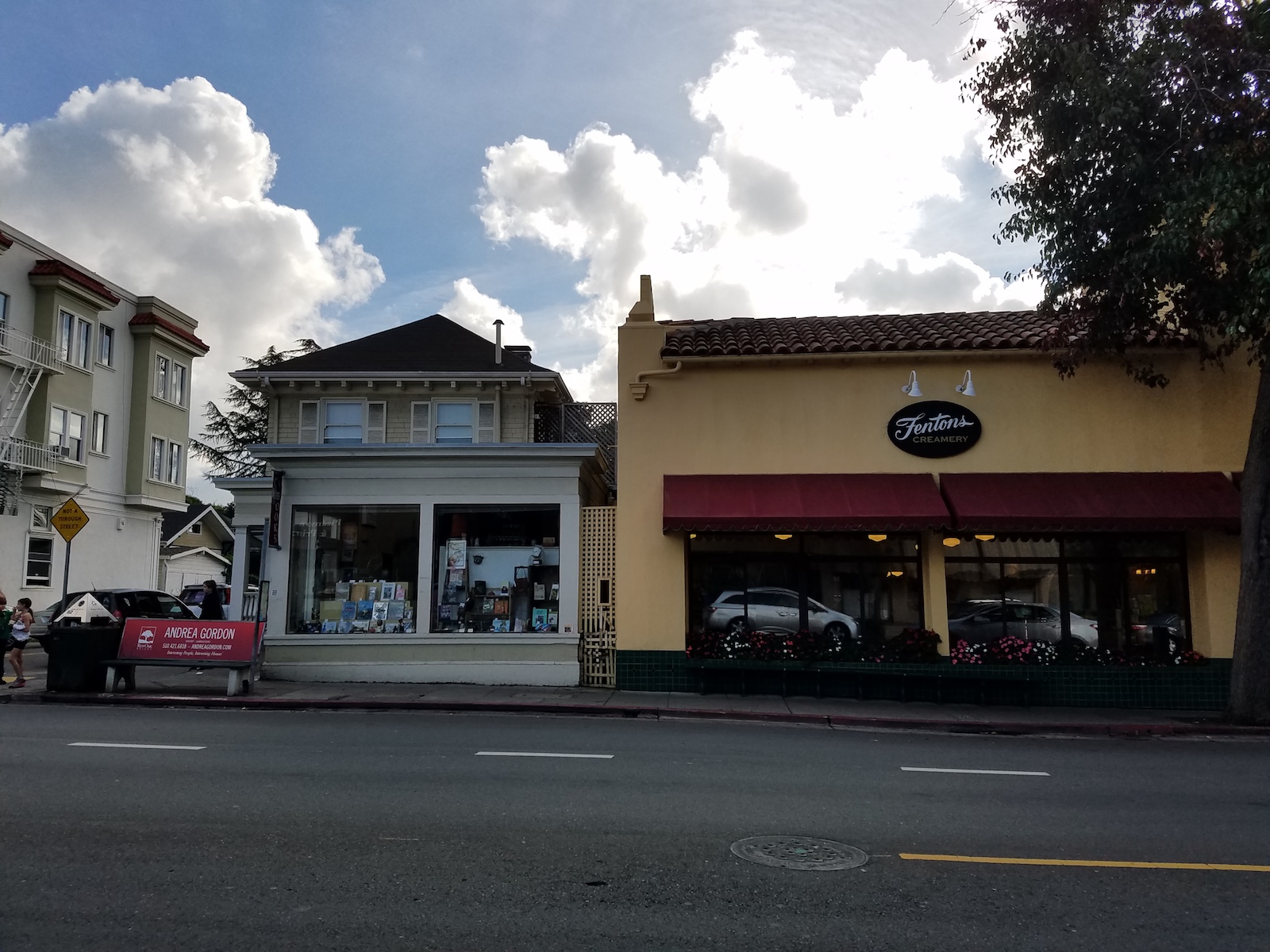
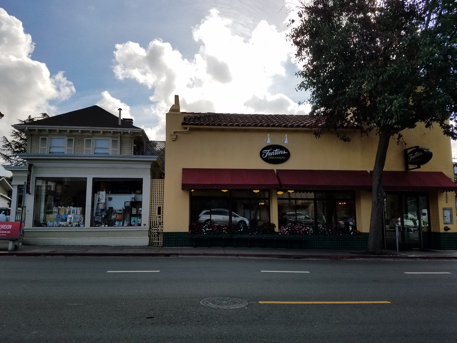
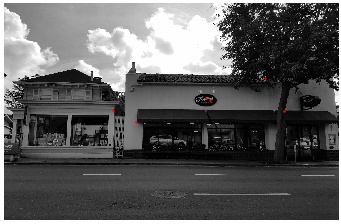
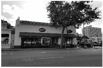
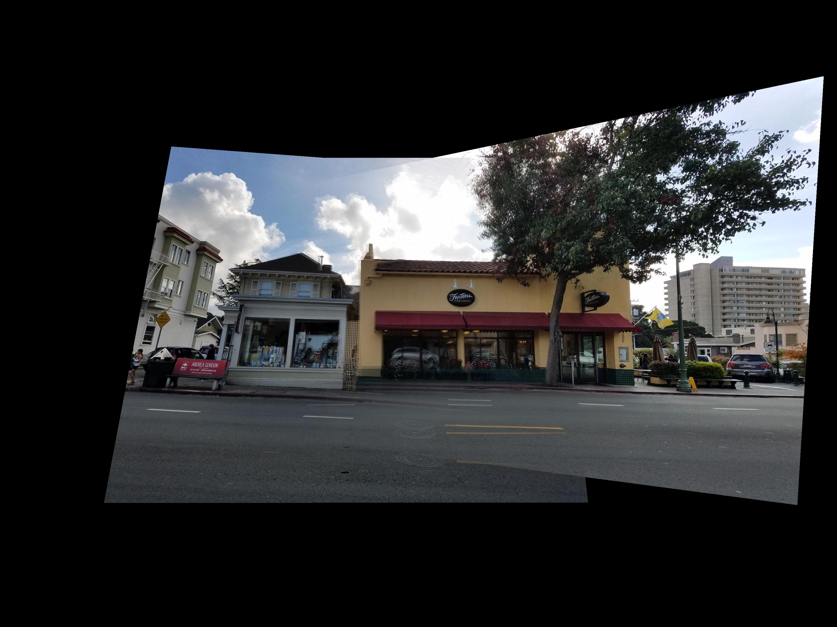
This is the first mosaic. The pictures were taken outside of Fenton's in Oakland.
 |
 |
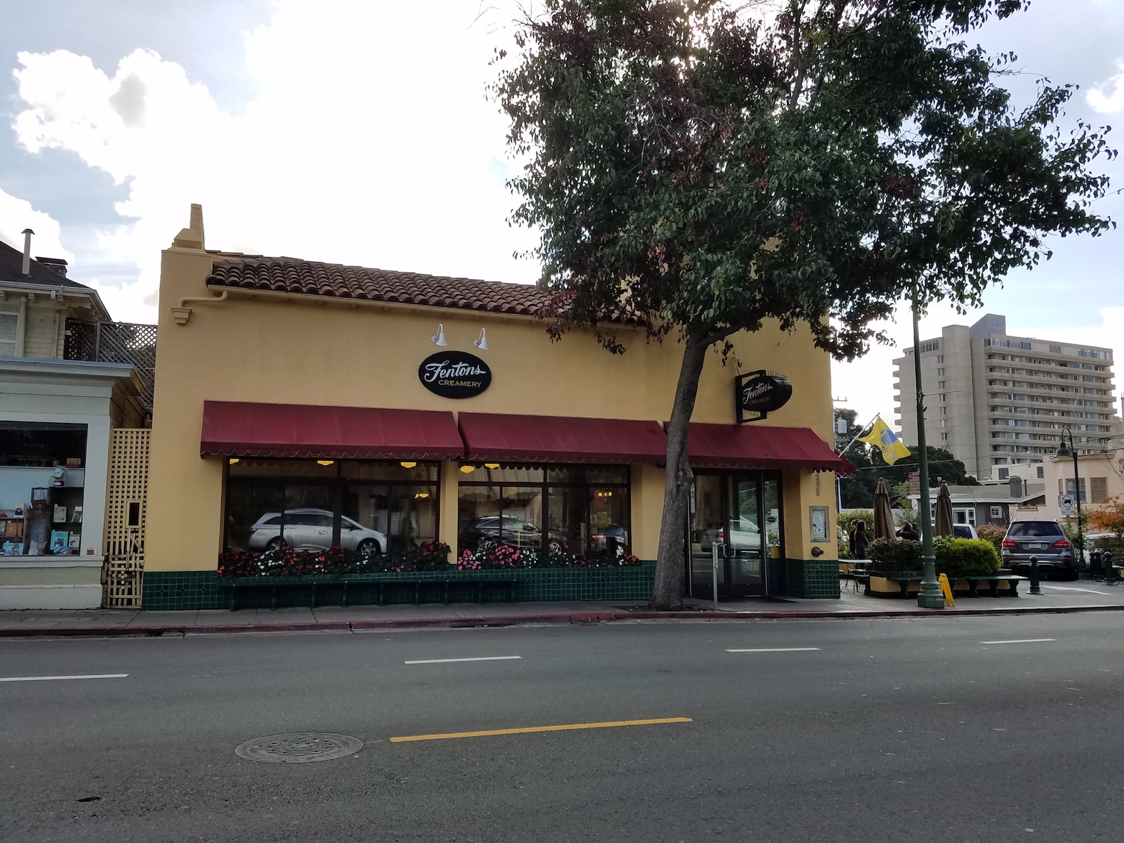 |
| Original image (left) | Original image (center) | Original image (right) |
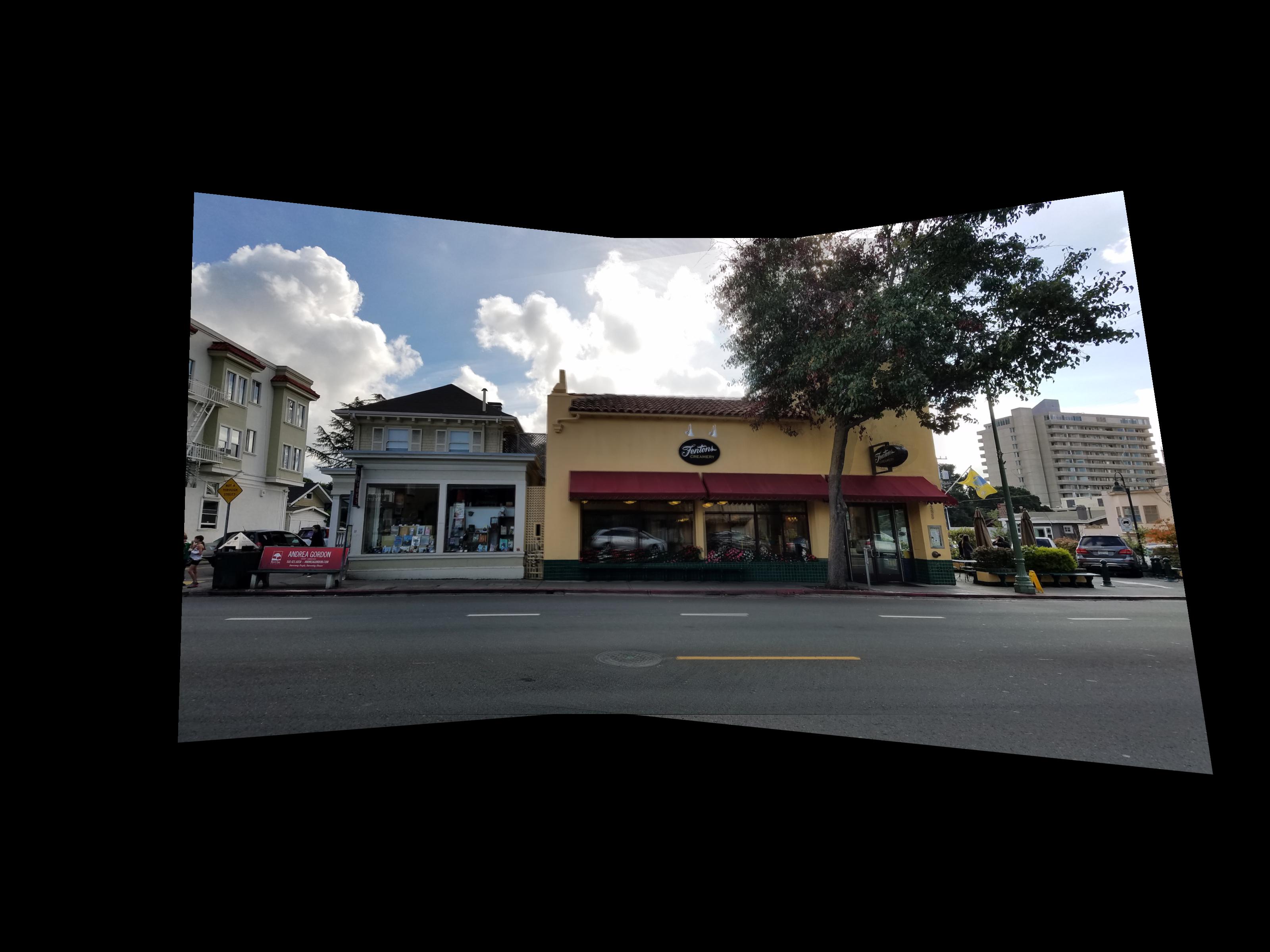 |
| Mosaiced image |
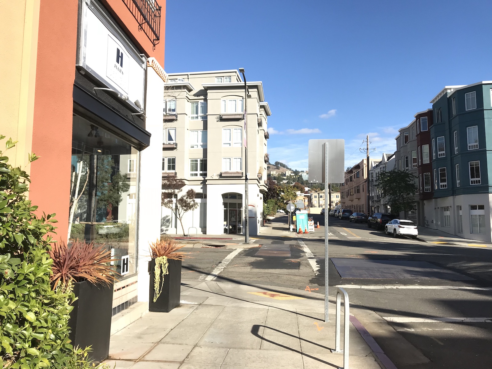
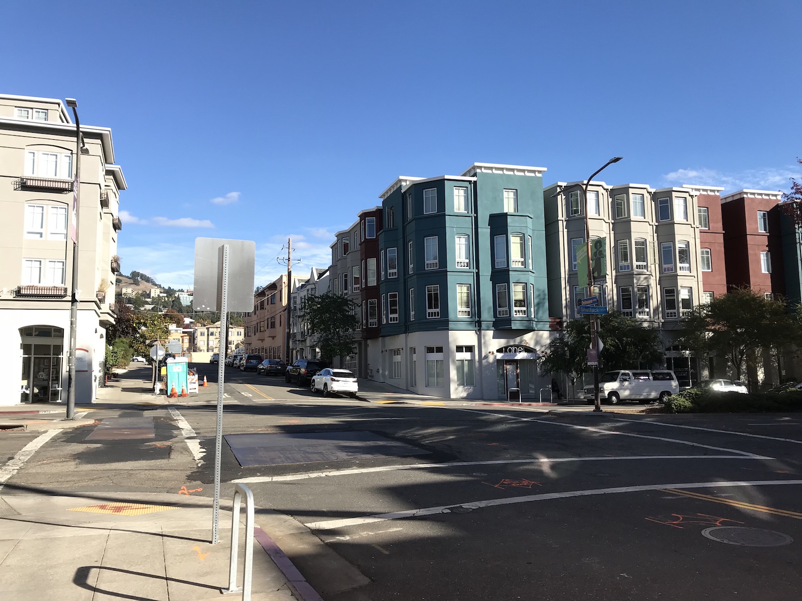
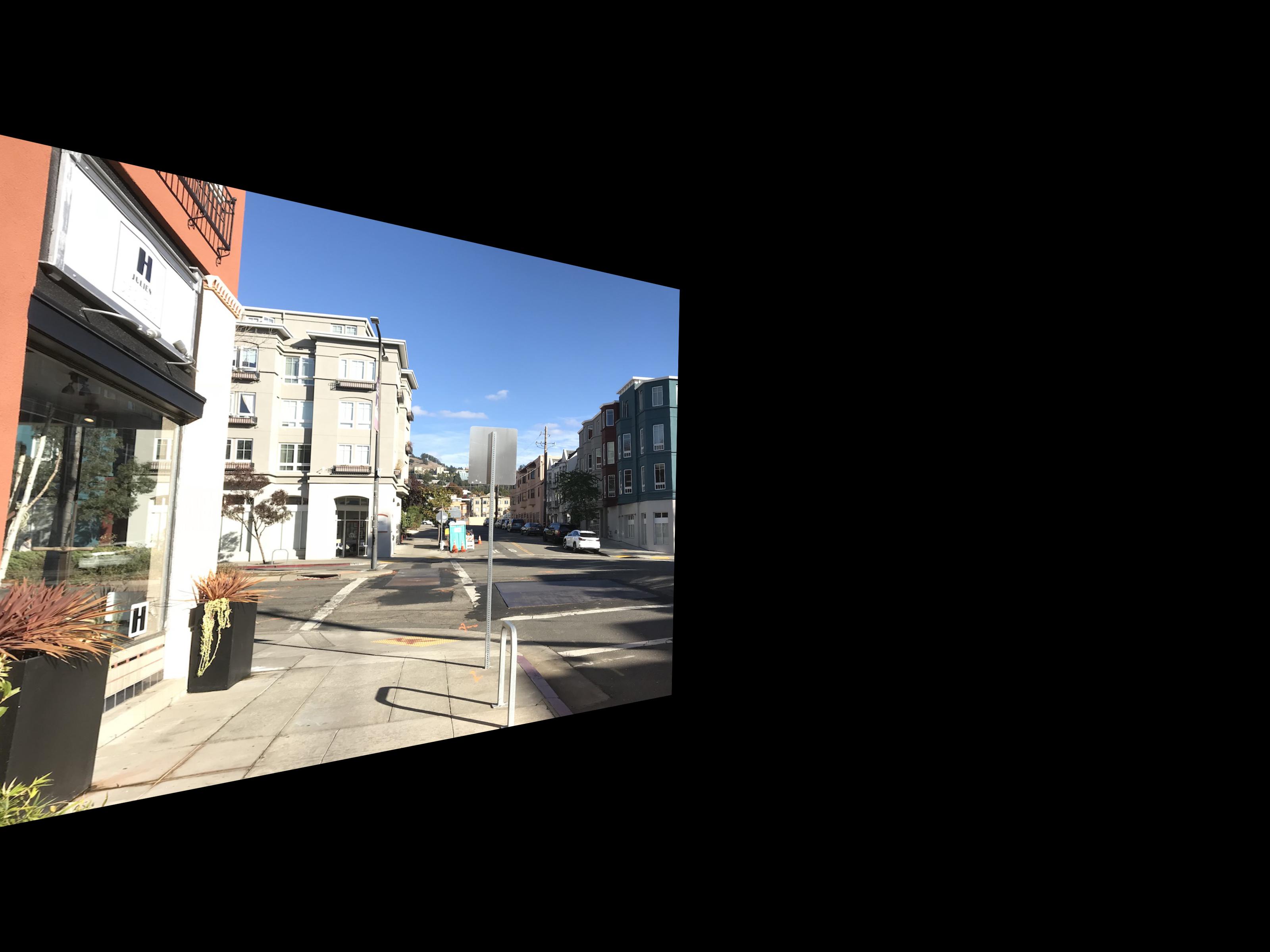
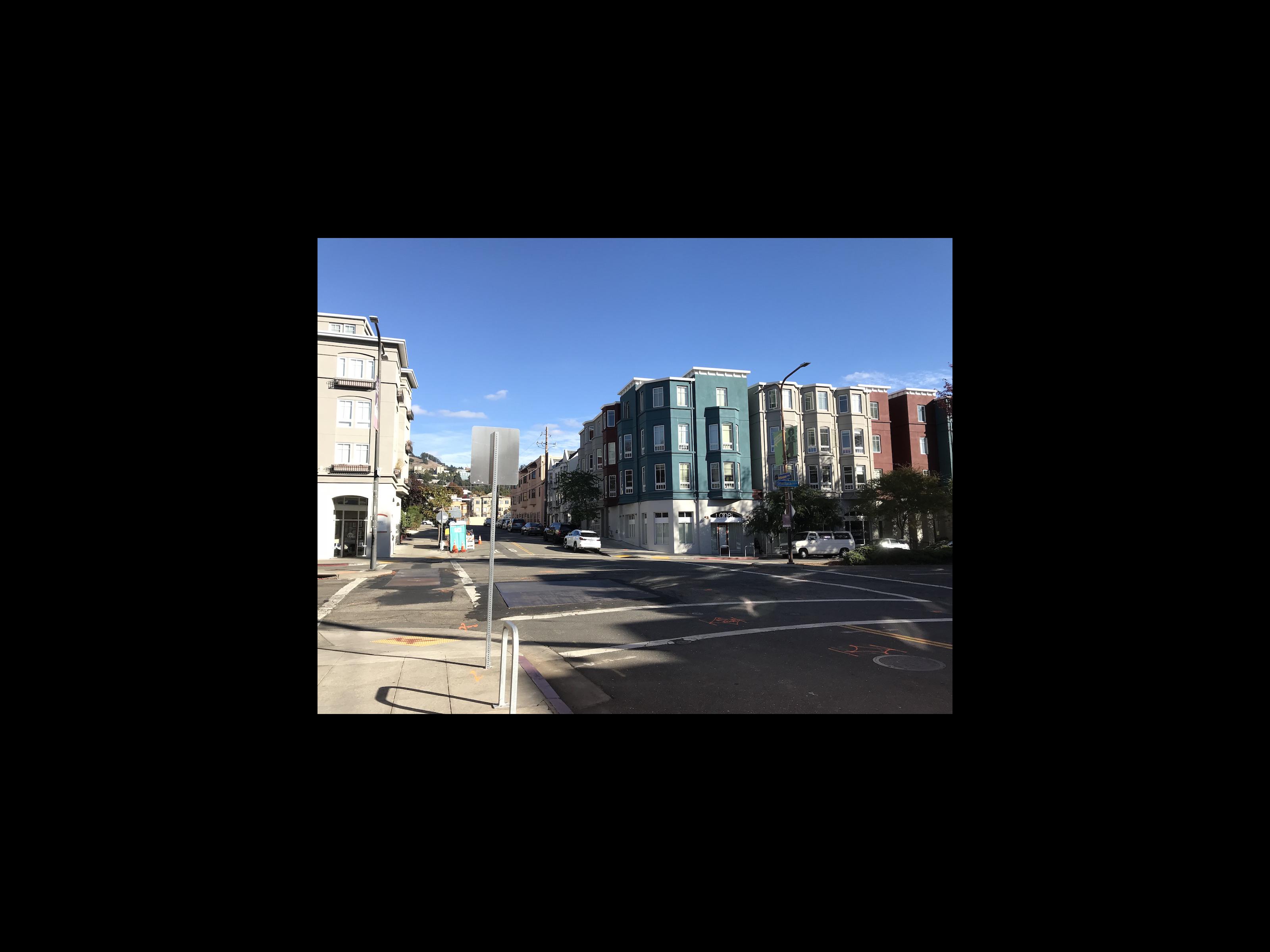
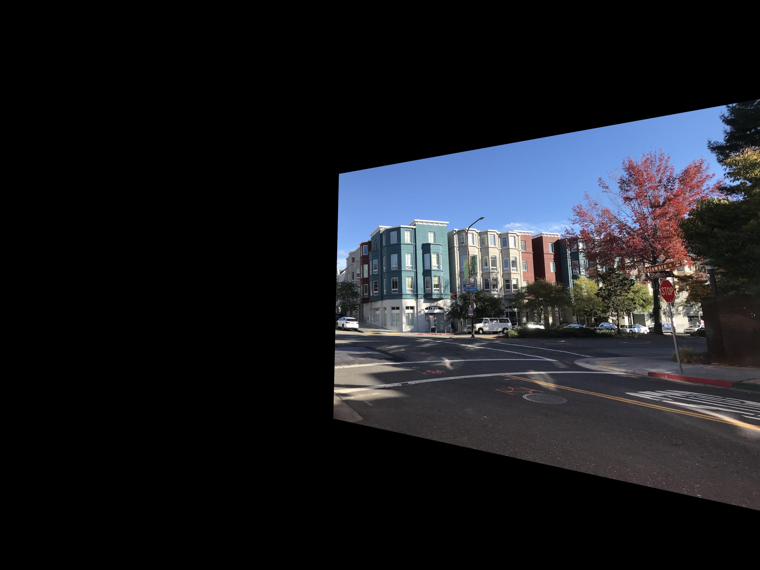
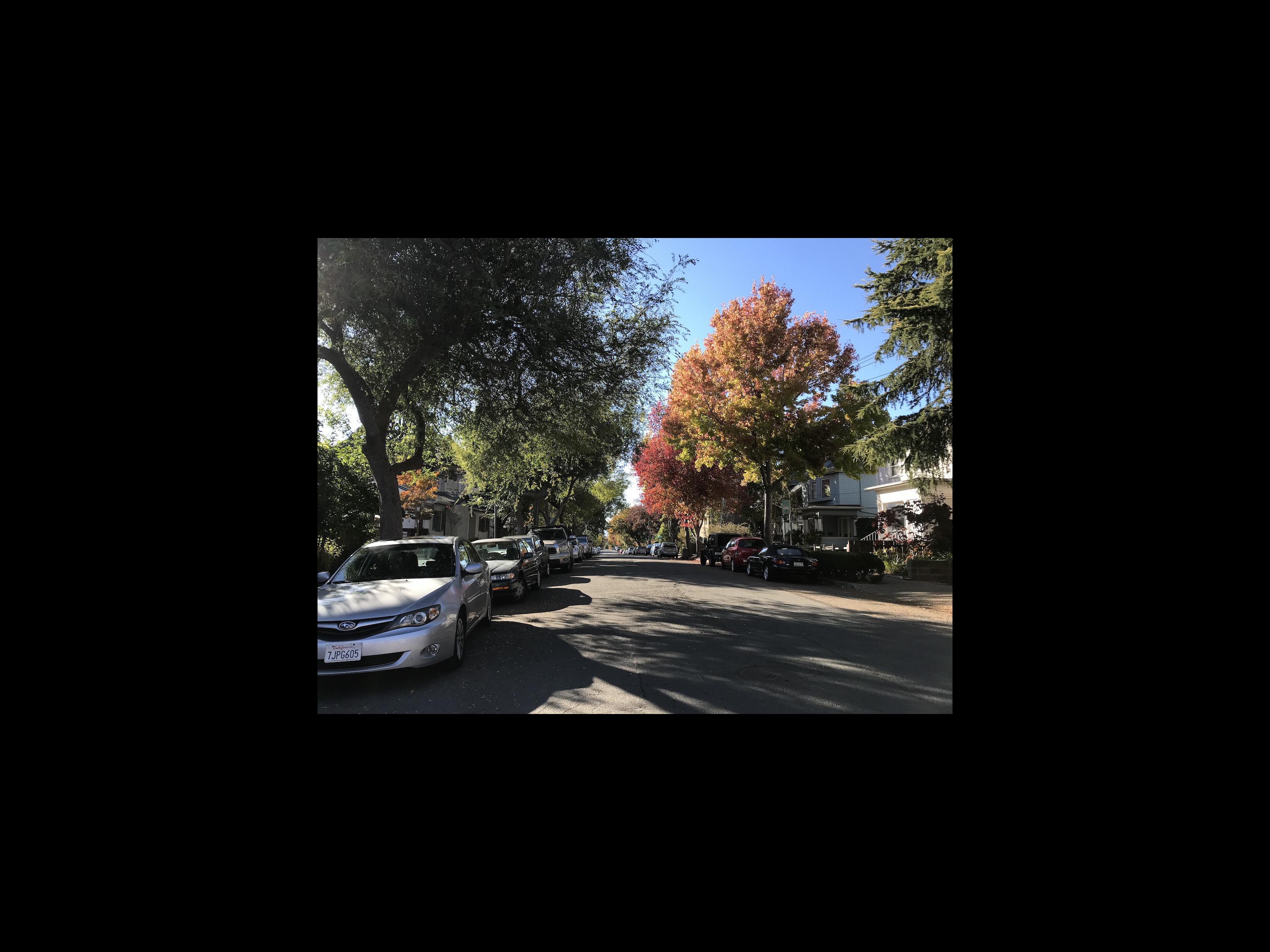
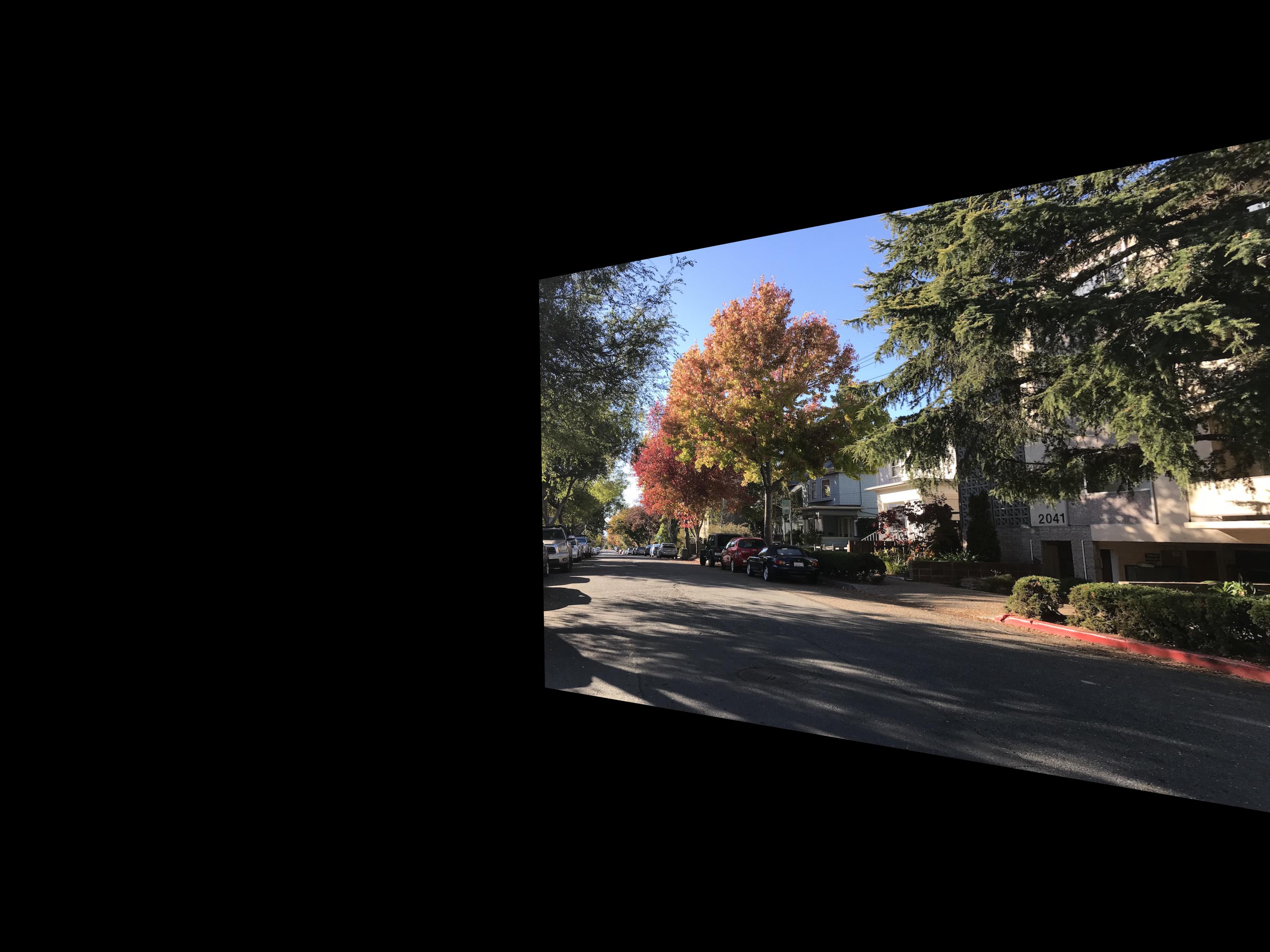
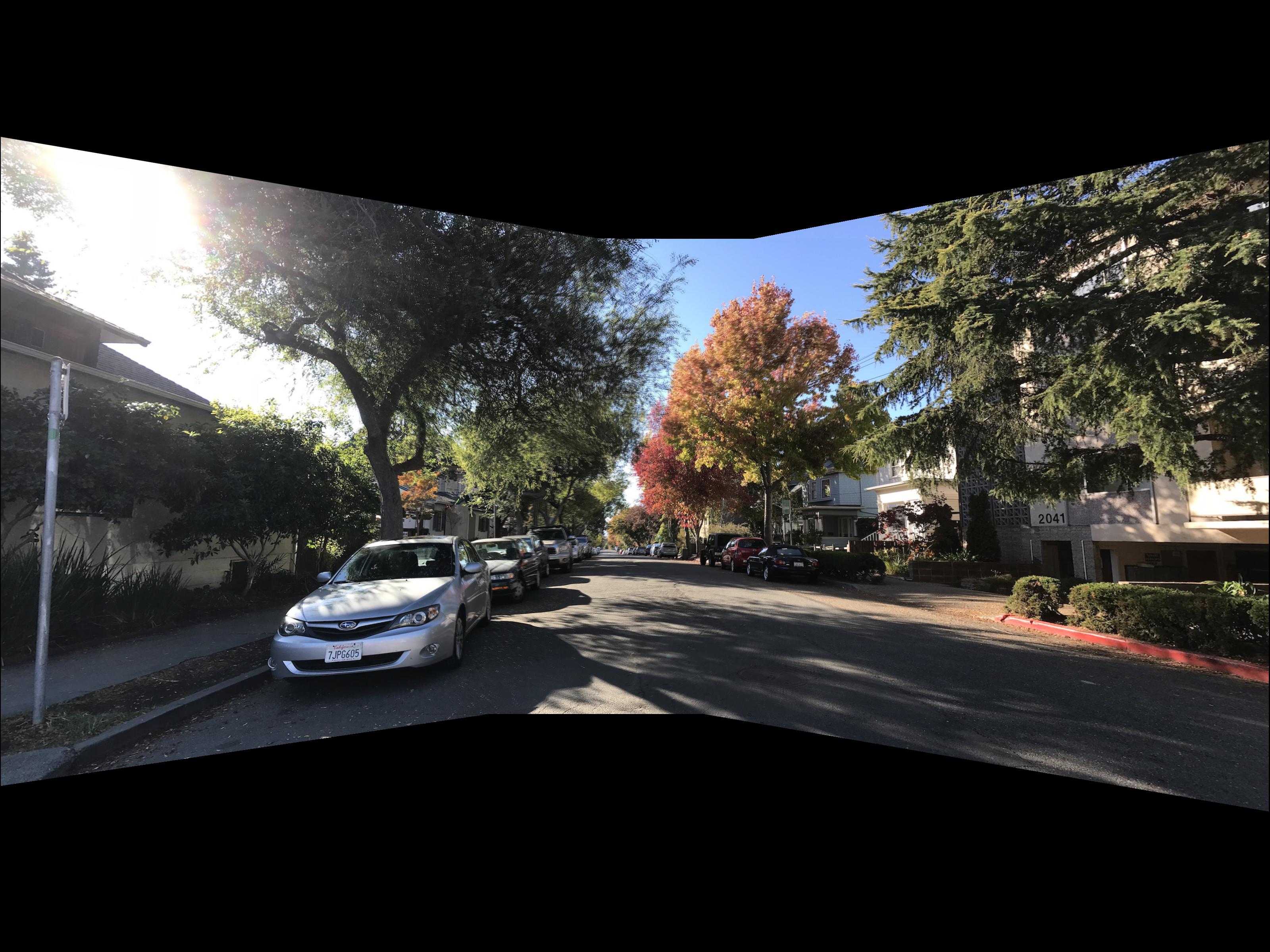
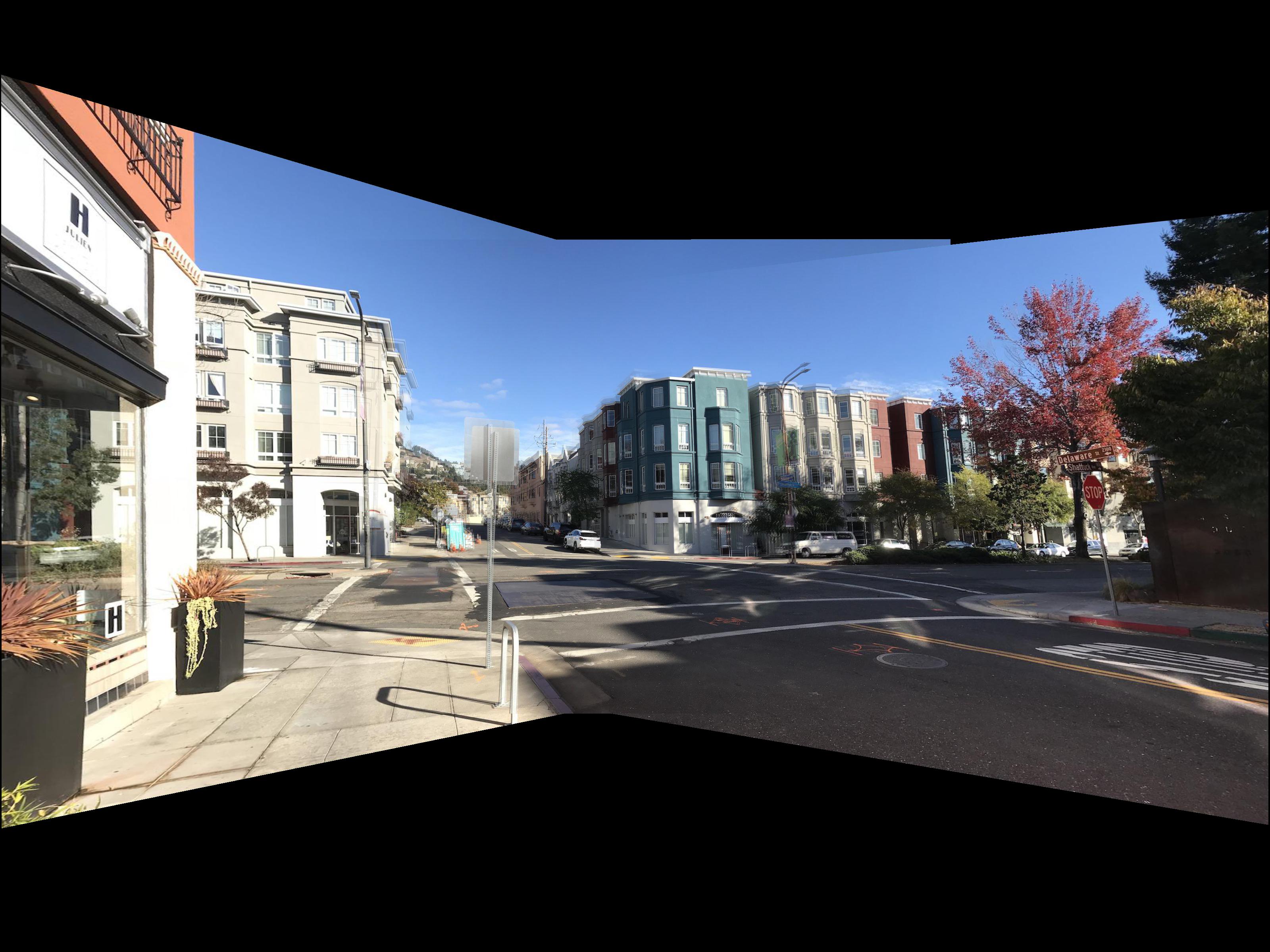
Here is the second mosaic. These images were taken near Northside in Berkeley.
 |
 |
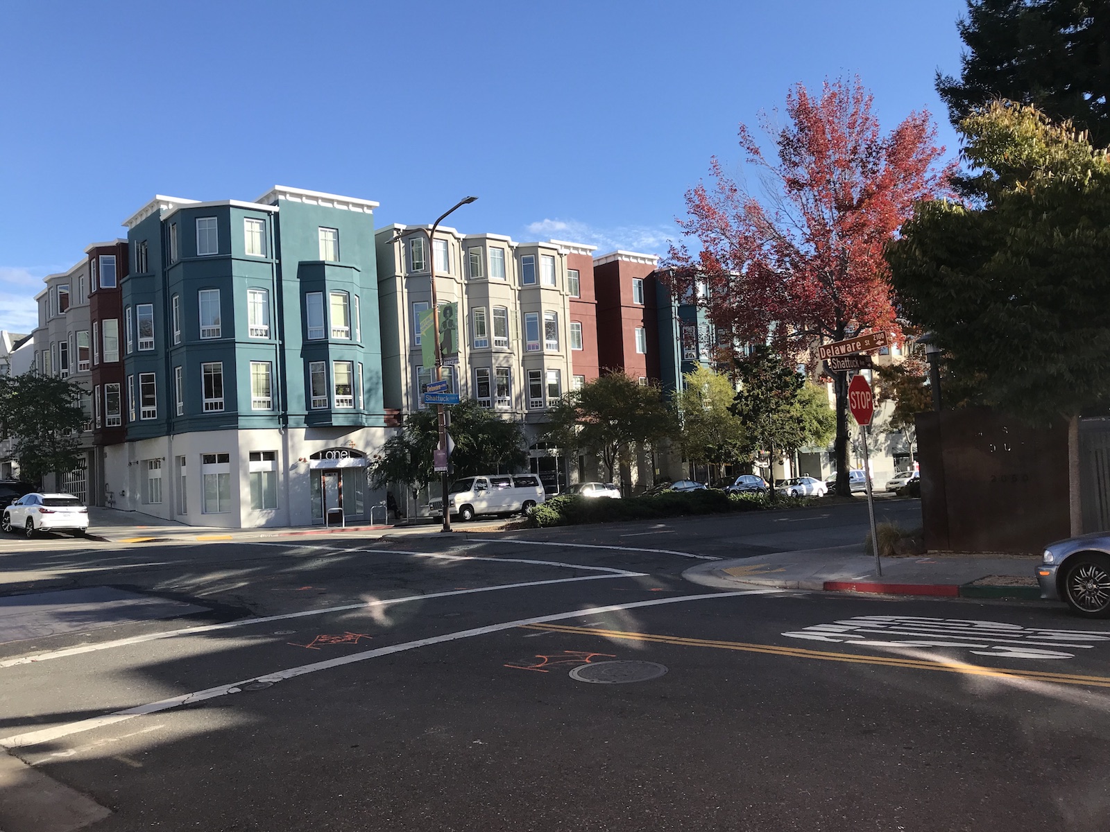 |
| Original image (left) | Original image (center) | Original image (right) |
 |
 |
 |
| Warped image (left) | Warped image (center) | Warped image (right) |
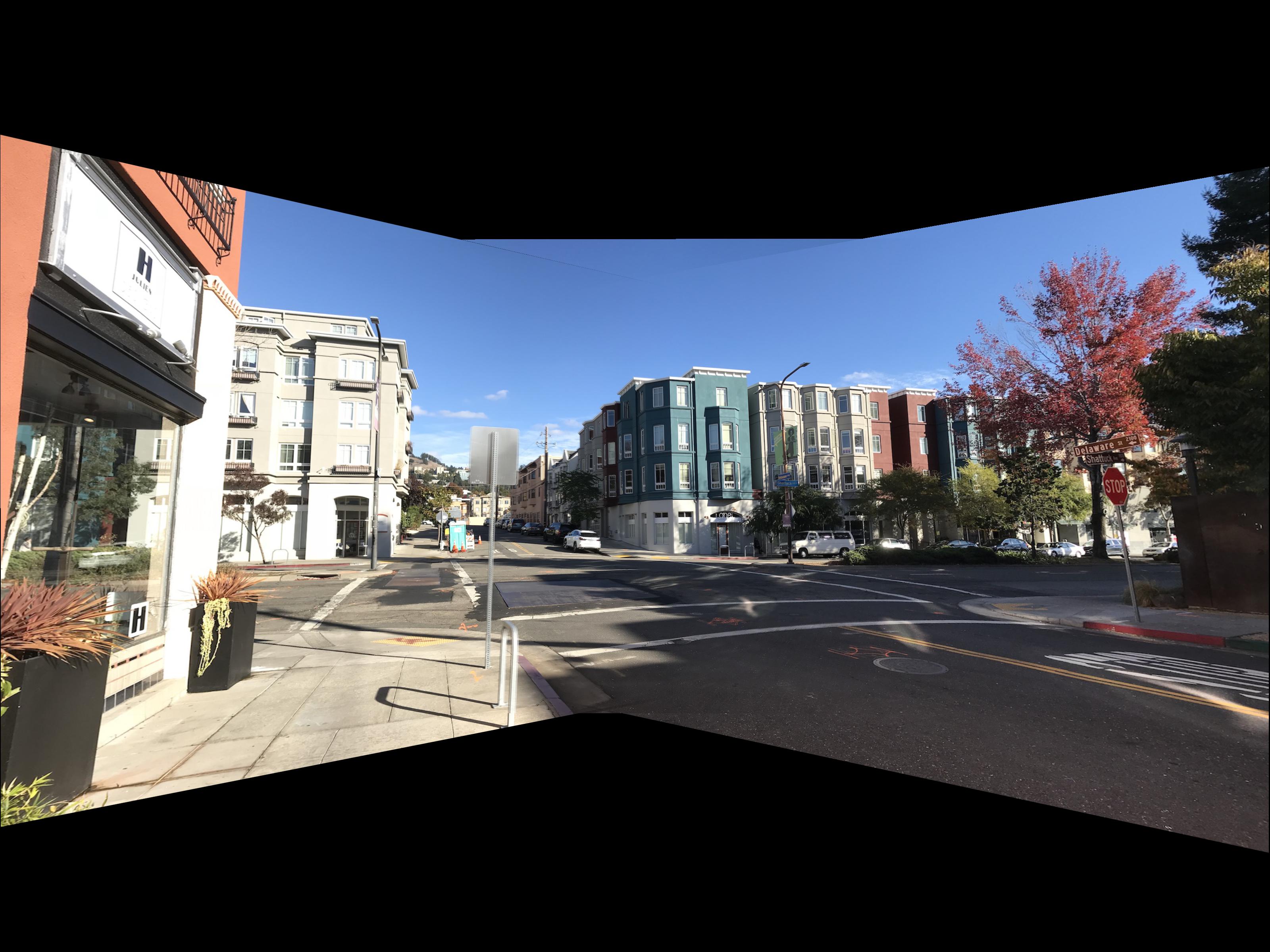 |
| Mosaiced image |
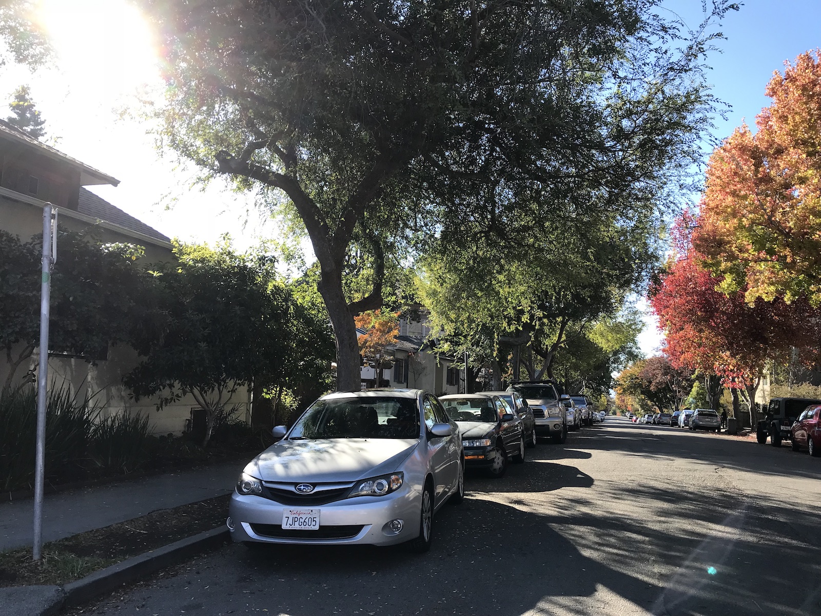
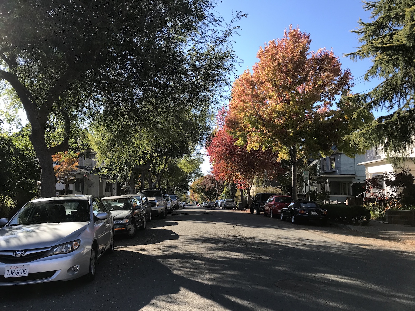
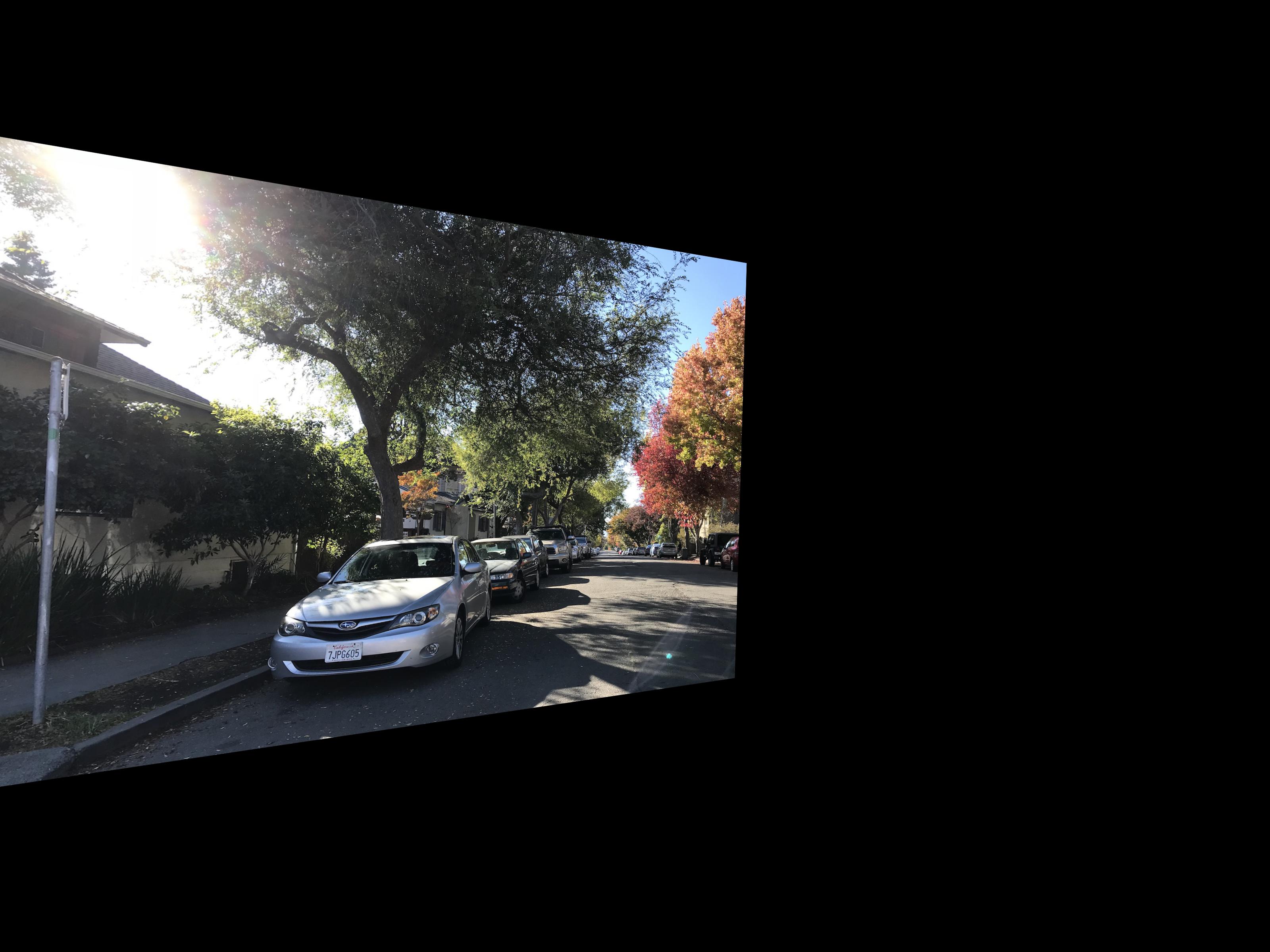
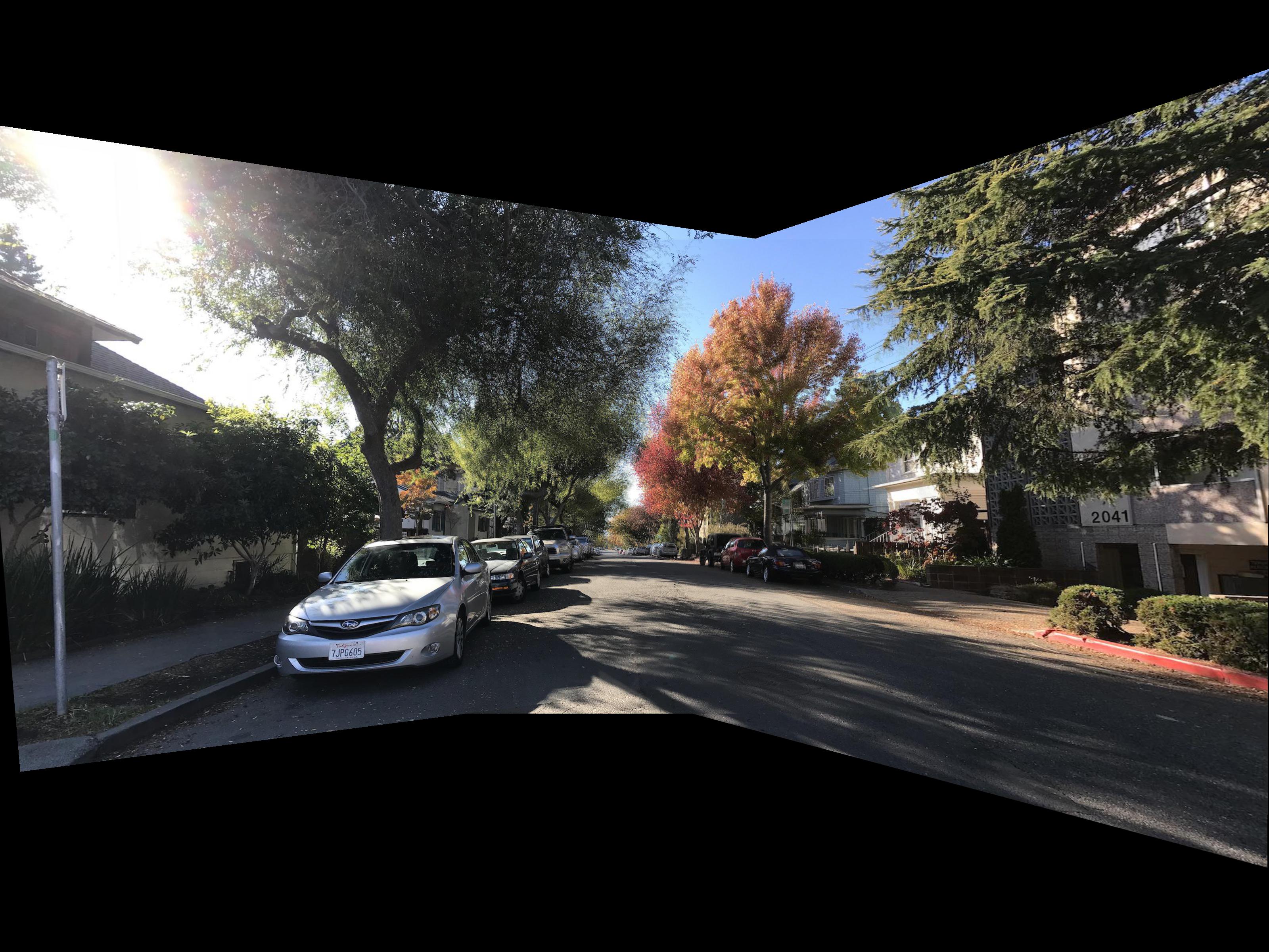
Here is the third and final mosaic. These were also taken near Northside in Berkeley.
 |
 |
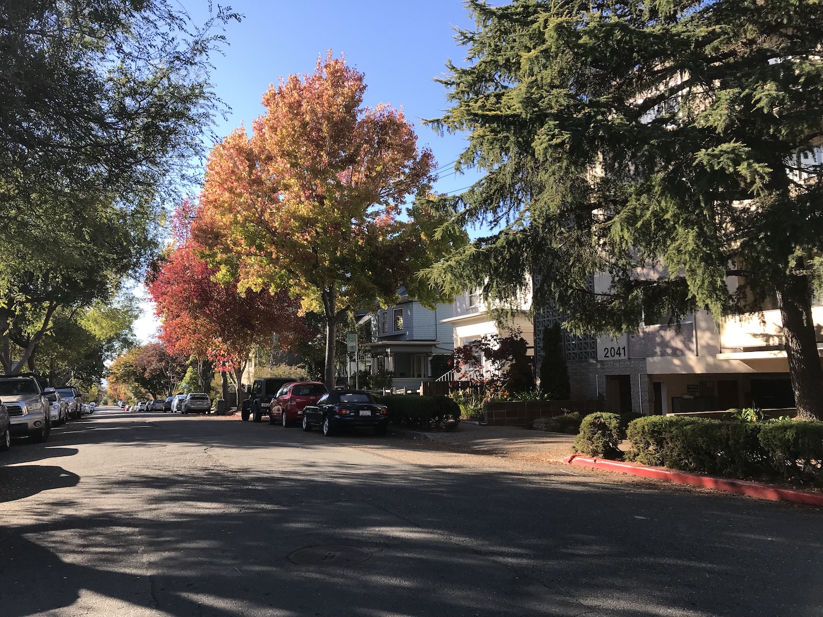 |
| Original image (left) | Original image (center) | Original image (right) |
 |
 |
 |
| Warped image (left) | Warped image (center) | Warped image (right) |
 |
| Mosaiced image |
This was a super cool project! I liked that it utilized basic linear algebra concepts to create stunning results.
The idea for this section of the project was to automate the feature selection process. This is broken down into several steps which are described below.
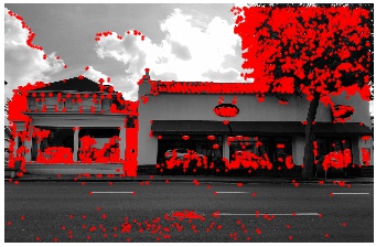
A Harris interest point is one such that if we move a window centered about that point in any direction, we would see a large intensity change. For each point, we can calculate an interest point value that gives us a notion of how "corner-y" a point is. The higher the value, the more "corner-y" it is. The following images are the originial images that we worked with and the Harris interest points thresholded to 0.1 (points with lower values were not included in the image).
|
|
| Original centered image of Fenton's | Original right side image of Fenton's |
 |
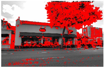 |
| Centered image of Fenton's with Harris IP's, threshold = 0.1 | Right side image of Fenton's with Harris IP's, threshold = 0.1 |
To make sure our feature points are well spread out, we will implement ANMS. Conceptually, we want to pick points from the previous step that are locally maximal. This depends on how large of a radius our neighborhood is. But we notice that once a point is defined as maximal in a neighborhood of some radius r, it is also maximal for all smaller neighborhoods r' < r . Now we can define the minimum suppression radius. This is smallest radius r_i such that a point i would be suppressed by (would have a smaller strength than) one of its neighbors. We can find these radii for each point and take the top n points with the largest radii. The images below contain the top 500 points selected with ANMS.
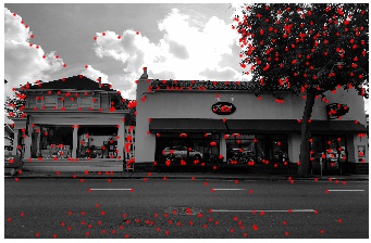 |
 |
| Centered image of Fenton's, top 500 points from ANMS | Right side image of Fenton's, top 500 points from ANMS |
Surrounding each interest point left over from the previous step, we look at the blurred 40x40 patch of pixels centered about that point. The feature that we keep for a given point is the downsampled [to 8x8] version of the 40x40 patch.
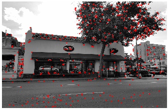
Suppose we have two sets of features from the previous step for two images that we want to match. For a given point in the first image, we can look at its corresponding feature vector and find the first and second closest neighbor feature from the second image. We then take the ratio of the squared distances 1-NN / 2-NN and store these temporarily. Once we have the ratios for all the points, we keep the ones that are below some predefined threshold. The reason for thresholding based on this ratio instead of the traditional squared 1-NN error is because there is a significant overlap between correct and incorrect matches when we only look at the 1-NN squared error. Below are images of the points selected as feature matches. In the examples below, we thresholded to 0.3.
 |
 |
| Centered image of Fenton's, features matched with right side image | Right side image of Fenton's, features matched with center image |
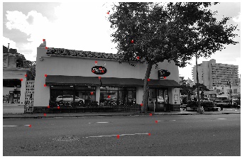
RANSAC allows us to iteratively find a homography between two images. First, we select 4 pairs of points at random and compute a homography from it. Then we evaluate how many pairs of points are correctly identified with our homography -- the correctly mapped points are called inliers. We continue doing this for until we get some number of inliers desired or we have reached a maximum number of iterations. At which point, we use the largest set of inliers from any single iteration to compute our homography. Below are images of points that were selected from the feature matching step after running the RANSAC algorithm on them.
 |
 |
| Centered image of Fenton's, inlier points after using RANSAC | Right side image of Fenton's, inlier points after using RANSAC |
The following are side by side images of mosaics created with hand selected features and the same mosaics created with automatically generated features.
|
 |
| Mosaic of Fenton's with handpicked features | Mosaic of Fenton's with automatically generated features |
|
 |
| Mosaic of North Berkeley corner with handpicked features | Mosaic of North Berkeley corner with automatically generated features |
|
 |
| Mosaic of North Berkeley street with handpicked features | Mosaic of North Berkeley street with automatically generated features |
Woooo lord this project was really cool. I really liked the ANMS section. I thought that it was a really clever way of framing the problem and I really enjoyed this section of the paper. I also found it amusing that RANSAC's algorithm is "guess and check for the correct homography", and how effective it actually is.
Styling of this page is modified from bettermotherfuckingwebsite.com.