William Choe Frank
CS194-26 Proj6B
Image Warping and Mosaicing Part A
Overview
The goal of this project is take two or more photographs and create an
image mosaic by registering, projective warping, resampling, and compositing
them. This is a 2 part project. For part A, we manually select corrispondence
points between the 2 images we wished to combine into a mosaic. In part B,
that process is automated. More detail about the steps to achieve automation
will be mentioned after talking about the manual corrispondence point creation step.
We will first discuss recovering homographies. Then we will show how
those recovered homography matricies H can be used to warp images. Finally,
we will then show how those warped images can be used to create a mosaic
using linear blending.
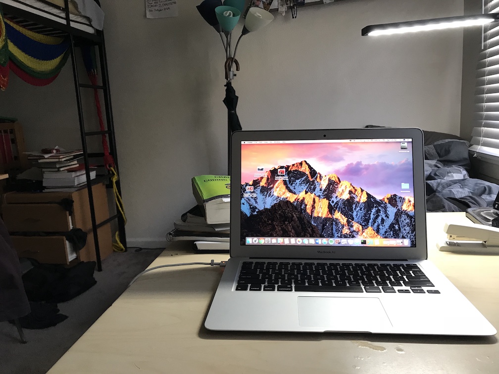
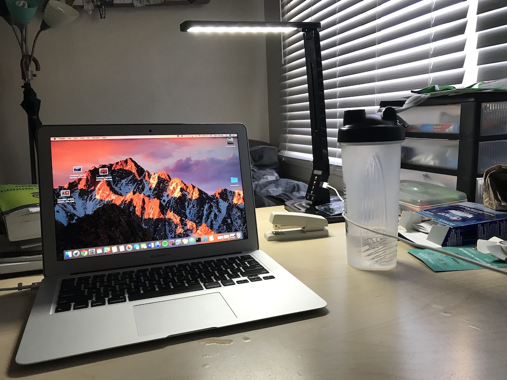
(Manual) Selecting Corrispondence Points
With the number of corrispondence points n being 4, we have enough
information to recover the homography matrix, which will be shown in the
next step, but in order to reduce noise and provide a more stable image,
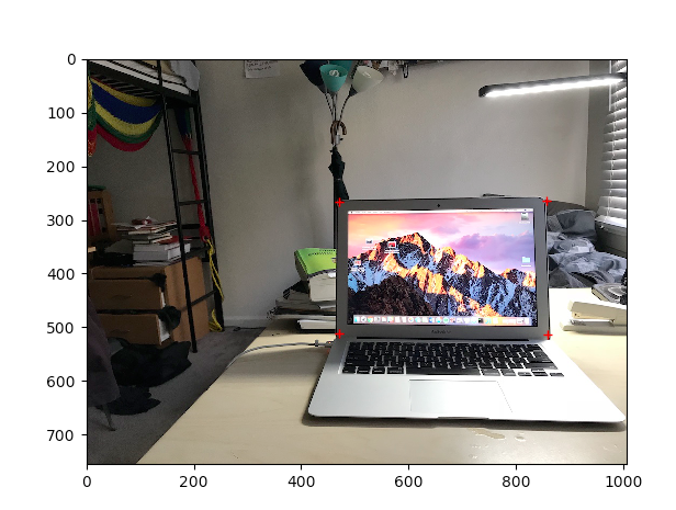
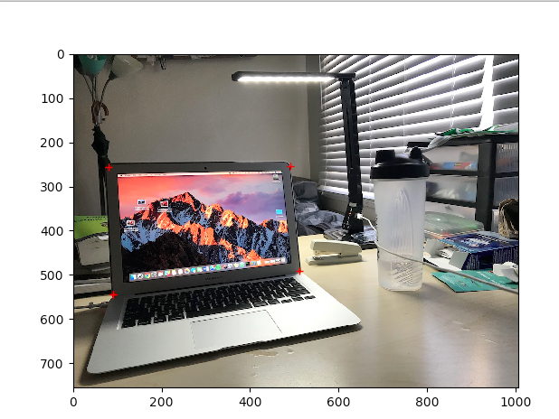
more than 4 points should be provided to make an overdetermined system.
Furthermore, points should be selected that corrispond to the same "object."
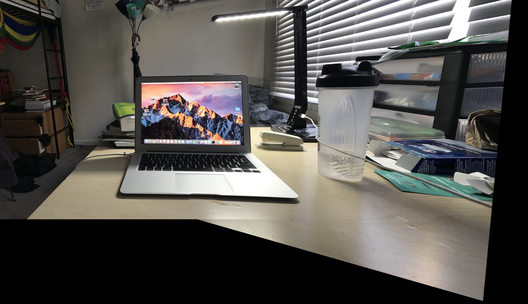
Below is an example of this with 2 pictures of my laptop on my desk.
Note: For showing rectified images, this is slightly different and will be
explained in it's own section
Recovering Homographies and Warping Images
The first step in creating a mosaic is to warp the images so they appear
to be on the same "plane". We can project an image imA to the plane of
a target image imB by recovering the Homography matrix H that captures
this transformation.
Computing the homography matrix for a projection of imA -> imB is as shown
by the matrix equation (Ax = b) below. Every 2 rows of A corrisponds to
a single corrispondence point where x_1, y_1 are the x,y coordinates of
the ith corrispondence point in imA, and x_1`,y_1` corrisponds to the x,y
coordinates of the ith corrispondnce point in imB.
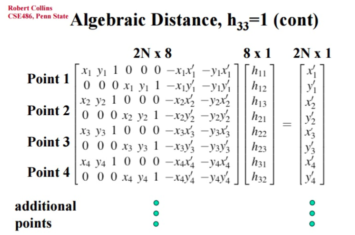
You can then use a least squares solver to solve for b which contains the
entries of the H matrix.
With H, you can project imA to imB. To achieve this, I used the inverse
warping technique that I used in project 4 to determine the new pixel values
of image A, imA`.
Image Rectification
Using H, you can project single images into different "views" by e.g.
clicking on four points that you know are a certain shape (i.e. square or
rectangle), then setting the next set of 4 points to a programmically
defined shape. In this case, imA and imB are the same image when computing H and doing warping,
but what differs here are the 2 sets of 4 corrispondence you select.
My results for this are below. The first image is the original
followed by the rectified image.
For this sign, we know that it actually represents a rectangle so rectify
the sign to show that.


For this table with drinks, we use the square pattern in the tile in
the upper table to rectify this image from a top down view.
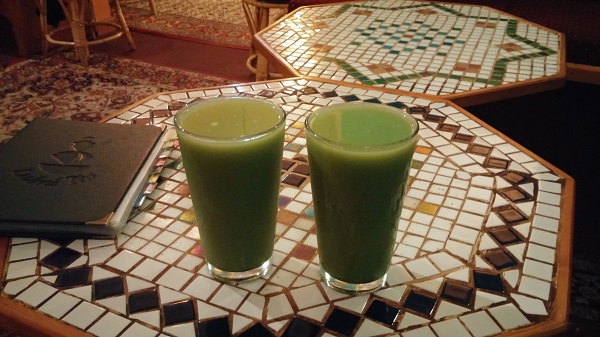
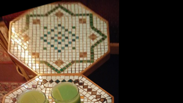
Image Mosaics
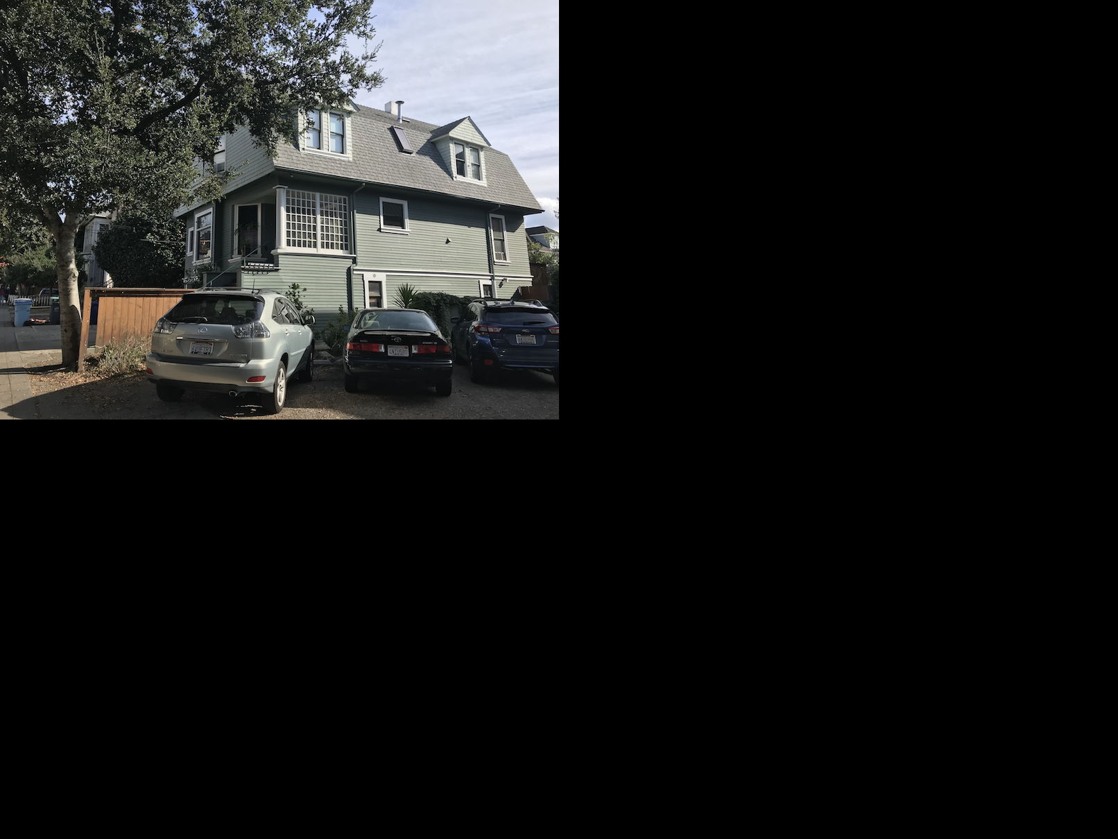
Here are 2 pictures of my neighborhood for which I will discuss creating
a mosaic for.
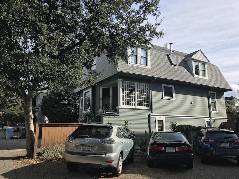
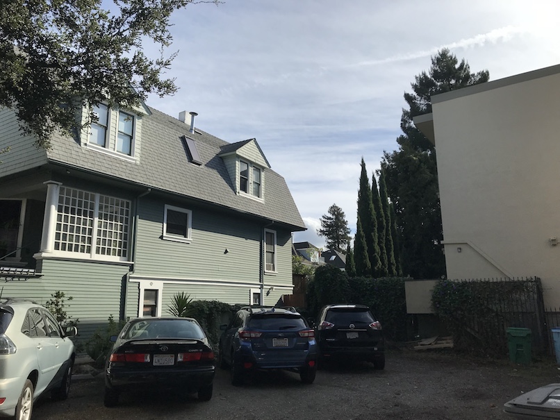
First, I selected my corrispondence points around the olive house in both images.
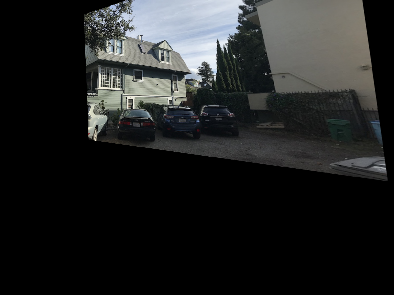
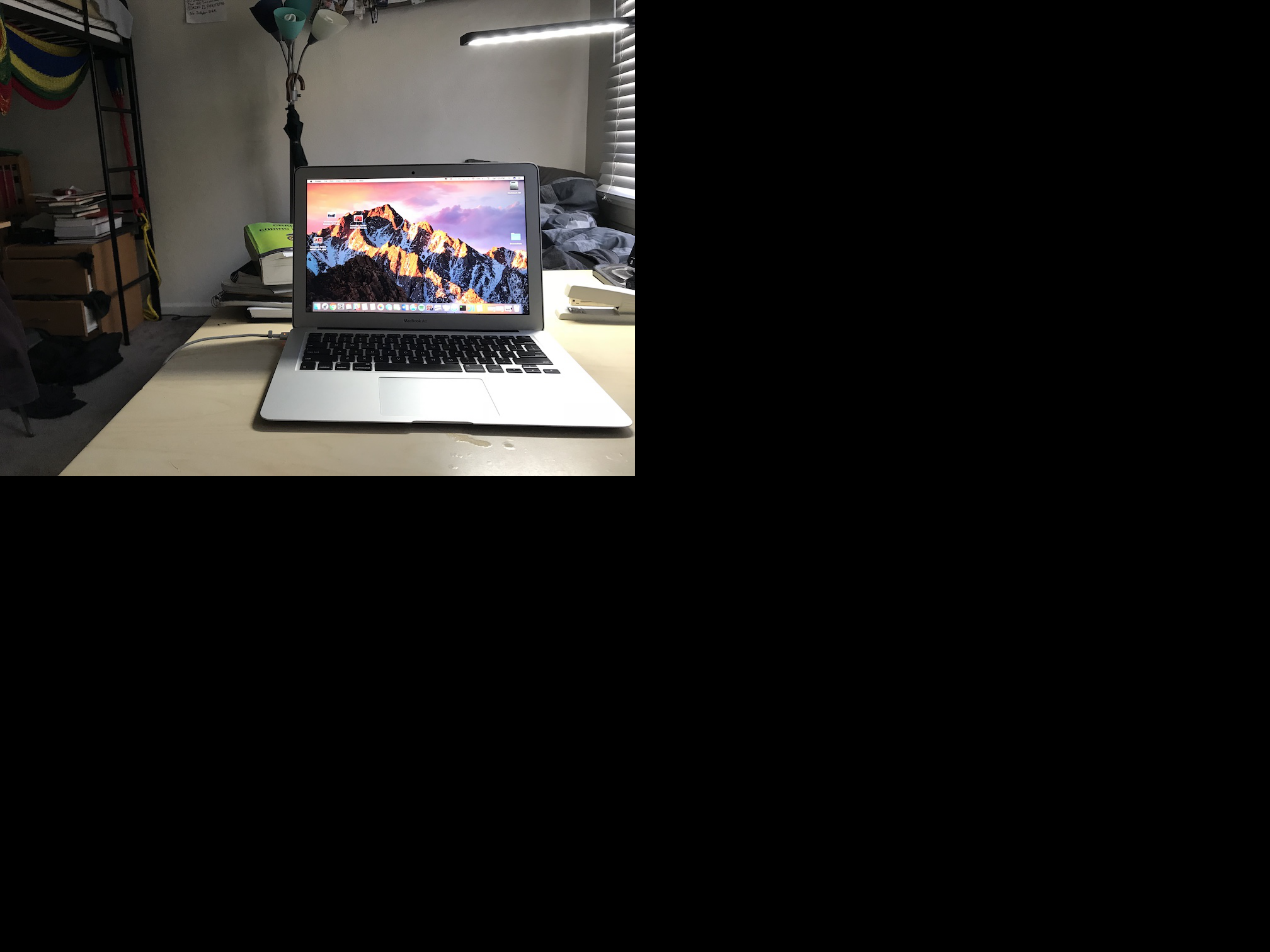
Using H and our warps of imA and imB computed in the previous part, we can
compute mosaics of the 2 images. We achieve this by warping imB to the
image plane of imA by using our computed H. Then we shift imA with respect to the warp that was
just done. So right now we have a shifted imA, imA` and a warped
imB, imB`.
imA` on the right; imB` on the left
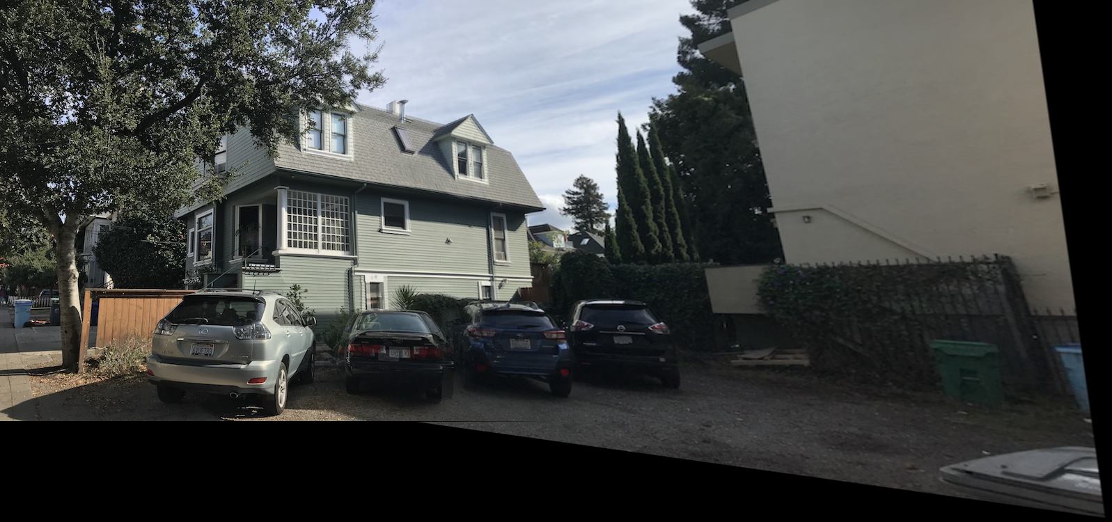
Now we can use linear blending to blend the 2 together.
Using a mask, and by using different alpha values depending on which image
I am closer to, I blend the 2 warped images together to finally produce
the mosaic (cropped).
Other Image Mosaics
My Desk
imA` on the right; imB` on the left
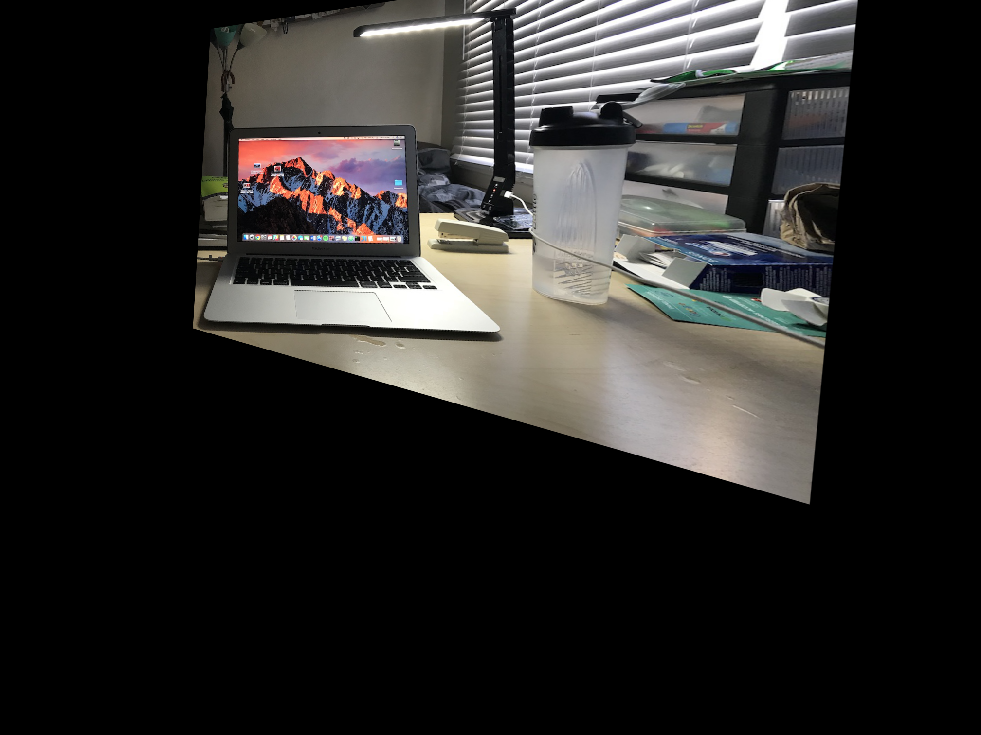
Desk Mosaic
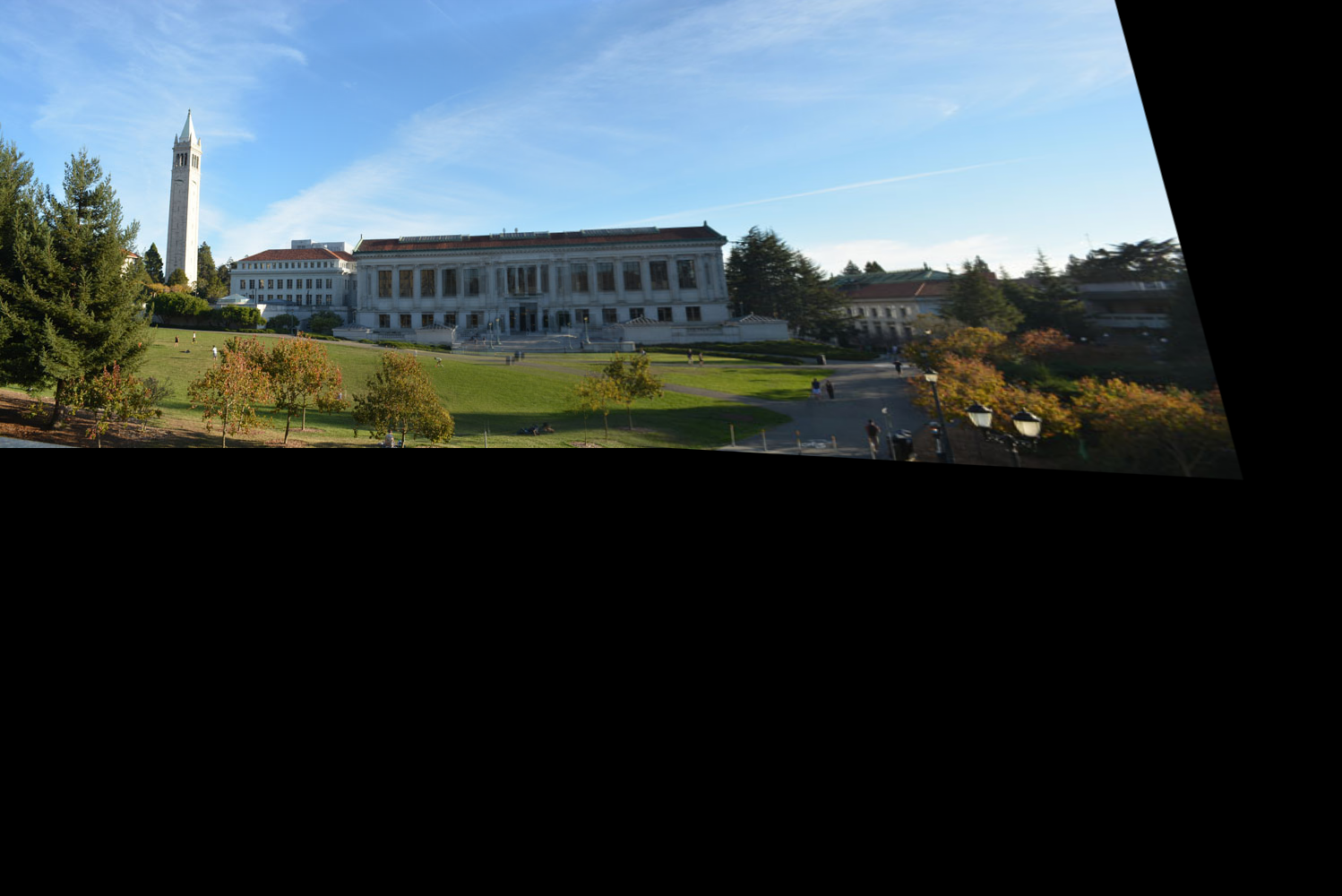
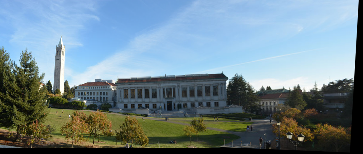
Memorial Glade
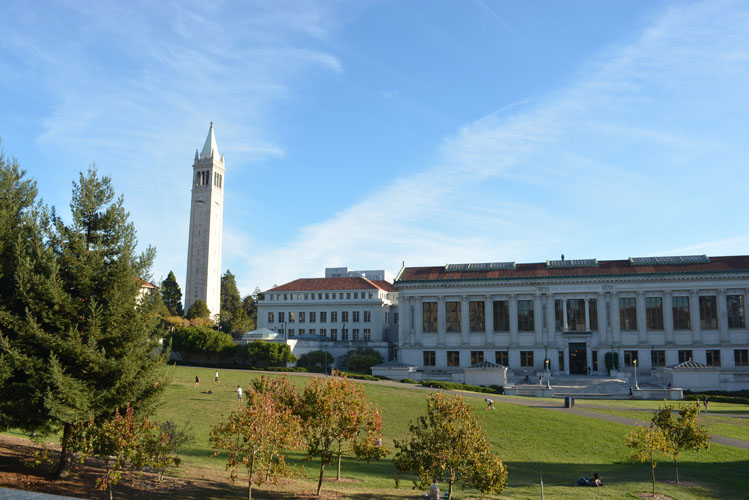
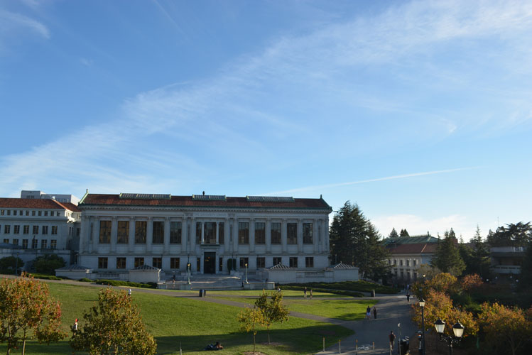
imA` on the right; imB` on the left
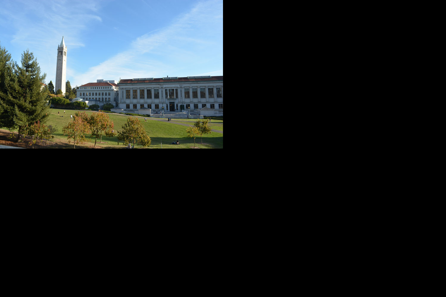
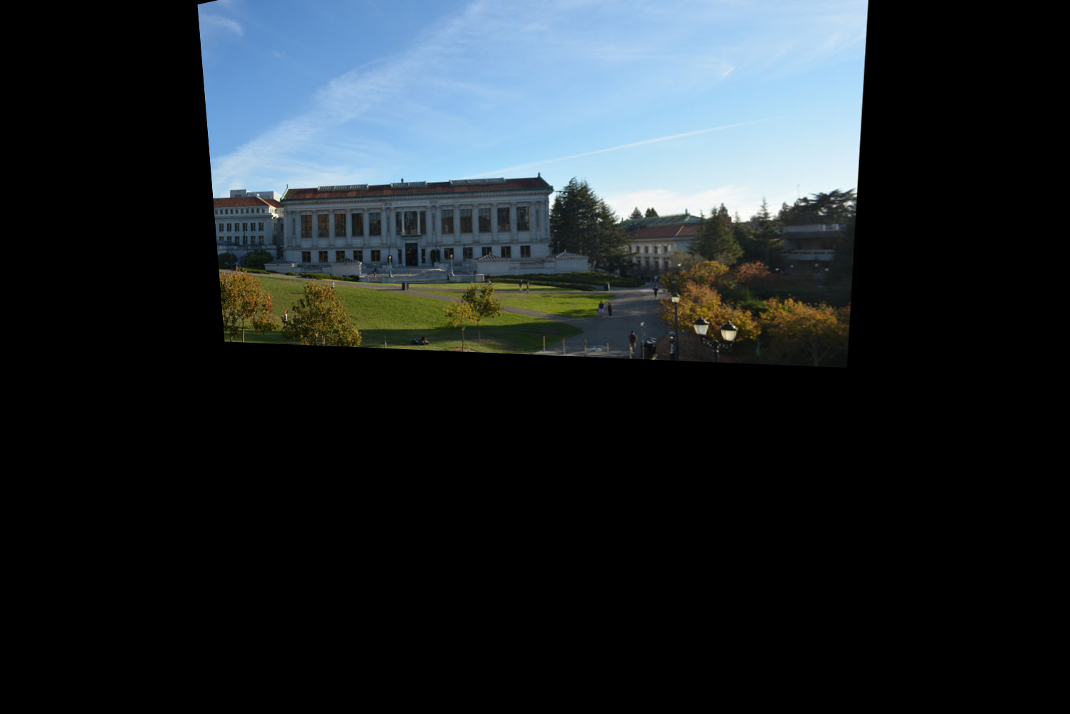
Desk Mosaic
What I Learned
I built on concepts that project 4 built (using linear algebra to use change
of basis matricies to project images to different planes). The coolest
thing about this part was that by applying foundational concepts from
linear algebra and photo computation, you can produce very good results!
I was most surprised at how well you can rectify images, and now I'm curious
what new information is already availble, and that cna be shown by rectifiing
an image to a different direction (e.g. maybe seeing something from a different point of view
in a crime case)
Part B
Overview
Defining correspondence points automatically is very involved. There are
4 main steps. The first is to detect "good" corners of the images. then
from those corners extract feature descriptors for those corners. After
that, we can try to match feature descriptors to create a mapping of features
between our 2 images. Once that is done, we finally use a method called
RANSAC to compute the homography matix, and once we get the homography matrix,
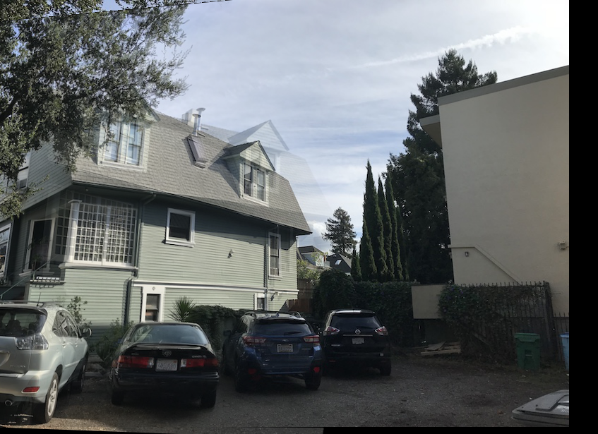
the steps are the same as in Part A. I will go into depth about each of these 4 steps
using the image of the lot behind my berkeley apartment.
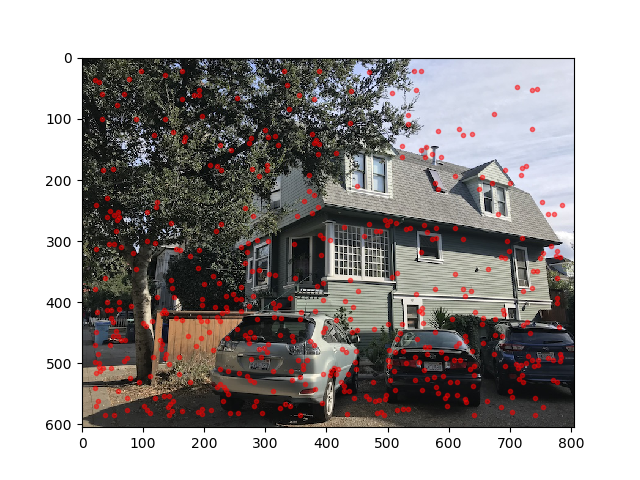
Corner Detection
To detect corners, I used the Harris Interest Point detector. But this detector
gives way to many points to do any meaningful computation so we need to reduce
this set down somehow. This is where ANMS comes in. The high level conceptual
idea of ANMS is that we only want points that are locally the best corner i.e.
Harris gives us a bunch of points around a corner where in reality we only
want 1 point there. So using ANMS as functionally described in the research
paper, I reduce from over 10,000 points to 500.
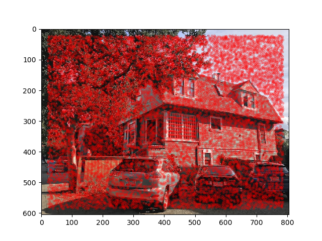
Harris Points from image 1
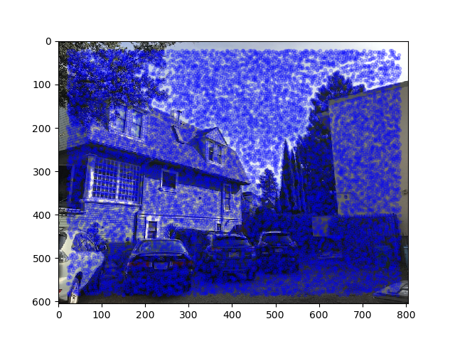
Harris Points from image 2
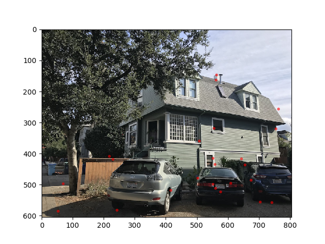
ANMS Points from image 1
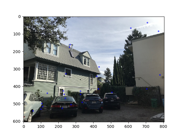
ANMS Points from image 2
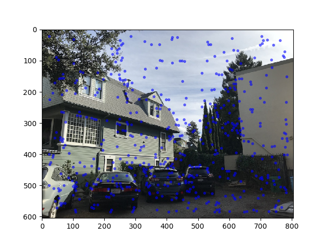
Image Alignment
So now we have good points from each image. Now we need to map featuers from
1 image to the other. We use Muli-Scale Oritented Patches as described in the paper.
Essentially, we gather the 40x40 grayscale surrounding each point, then downsample to
an 8x8 patch, then normalize. We do this to each point to get descriptor vecotrs for
each ANMS point.
Now to match features, as described in the paper we can use Lowe's technique.
For every feature vector, we compute its distance to all the other feature
vectors. We want the closest two features from the other image, NN1 and NN2.
We want to keep the feature vectors such that their NN1/NN2 ratio is less than some threshold.
This varried for me for each image. If the point exists in the second image,
the ratio is more likely to be closer to 0, otherwise the 1-NN/2-NN ratio will likely be close to 1.
Below are my images w/ the feature matching points. These points are all candiates to
be points for our Homography Matrix.
Though, there are still some outliers. To deal w/ this, we use a method
called RANSAC. Essentially, we iterate (i did 10,000) and over a set number
of times, we randomally select 4 points from 1 image to be the inputs for
calculating our H matrix. Note: we know the supposedly corresponding points
in the 2nd image from when we did feature mapping above and built a map
from one feaure in image 1 to a feature in image 2 (note this map is not necisarily one to one, which is why we need to do this a lot of times).
We choose the Homography which gives us the most inlier points as in features from
our feature map match up to where they ought to be after applying H to them. I do
this by using the good old distance formula (L^2).
Feature Matching points from img 1
Feature Matching points from img 2
Final Automatic on left, manual on right
Other Results, auto on left, manual on right