Feature Matching for Autostitching

Jacob Huynh
CS 194-26: Image Manipulation and Computational Photography
Professor Alexei Efros

Overview

The previous part of the project explored the idea of warping and mosaicing images together once we define the correspondence points manually. The goal of this project is to generate automatic correspondence points in order to achieve autostitching of multiple images. So, instead of having to identify features which correspond to each other manually, we can automatically detect similar features to generate accurate correspondence points. This would also theoretically create better stitched images, as the program would be able to detect much more correspondence points than one can detect manually.

Part 1: Harris Interest Point Detector

First, we need to understand that corners are the easiest to detect part of an image. So, the first correspondences we will use to identify features will be corners. In this project, and as is described in the research paper we will be following, we will use Harris corner detectors to detect corners in images. The Harris corner detector has already been nicely implemented fo rus in t he skeleton code, so we will use that to generate a set of Harris corner coordinates and a corresponding H matrix to all the coordinates which describe the pixel intensity h of each corner.

computer1 harris points

computer2 harris points

Part 2: Adaptive Non-Maximal Suppression

Because Harris corner detector detcts and outputs the corners of images indiscriminately, we need some way to reduce the amount of features to be more computationally feasible. A naive approach would be to simply choose the points in the descending order of corner response. However, doing this would create a tendency for points to cluster in small areas. So, as described in the research paper, we will use adaptive non-maximal suppression to find an evenly distributed set of feature points. For each point p_i, we find r_i, such that the distance to the closest point has significantly (as described by c_robust) higher value than p_i.

r_i = min|p_i - p_j|

f(p_i) < c_robust * f(p_i)

Finally, we choose the feature points to keep in descending order of r_i.

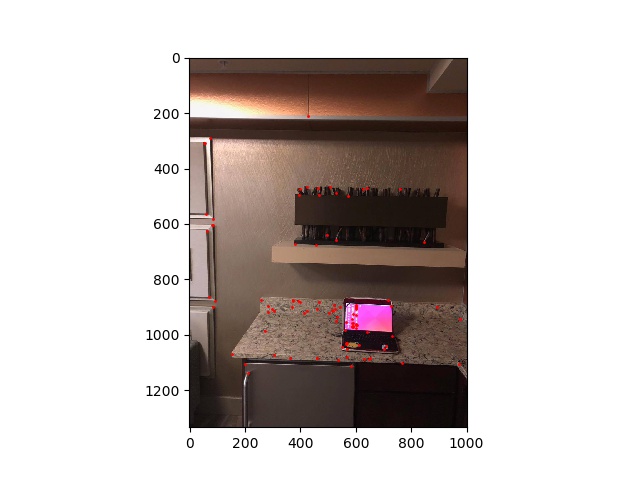
computer1 amns points

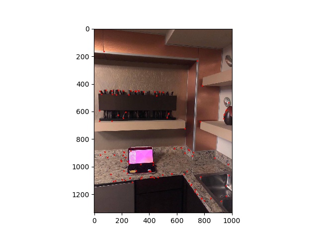
computer2 amns points

Part 3: Feature Descriptor Extraction Utilizing Multi-Scale Oriented Patches

After choosing the feature points, we need some way to compare the feature points of one image to another image, so that we can form correspondences between two feature points. In order to do this, we utilize Multi-Scale Oriented Patches, as described in the research paper. The idea behind MOPS is that we create a hashing scheme for patches of pixels centered at the feature point. This hashing scheme can then be used to correspond feature points which have similar hash values. For MOPS, we first choose a 40 x 40 patch centered at the feature point, then we subsample to the patch by 0.2, to have an 8 x 8 patch. Now that we have our feature patch, we need to create the hashing scheme. The hashing scheme recommended in the paper is to normalize the patch by subtracting the patch's mean, then dividing this difference by the standard deviation of the patch. Finally, we flatten this output to a feature vector of dimension 1 x 64.

Part 4: Feature Matching

Now that we have a feature descriptor, we now simply need to compare the hash values (feature vectors) of each feature point to each other to establish correspondences. We can compare them by using the dist2 function provided for us in the skeleton code, or alternatively utilize sum of squared distances (SSD) between two vectors. We will compare every vector in image 1 to every vector in image 2, saving both points only if the point with the best patch (1-NN in the paper) is significantly better than the second best match (2-NN). The way we define if 1-NN is significantly better than 2-NN is if (1-NN)/(2-NN) < epsilon, where epsilon is the error threshold we input. For all the images, the error threshold set is 20.

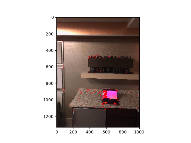
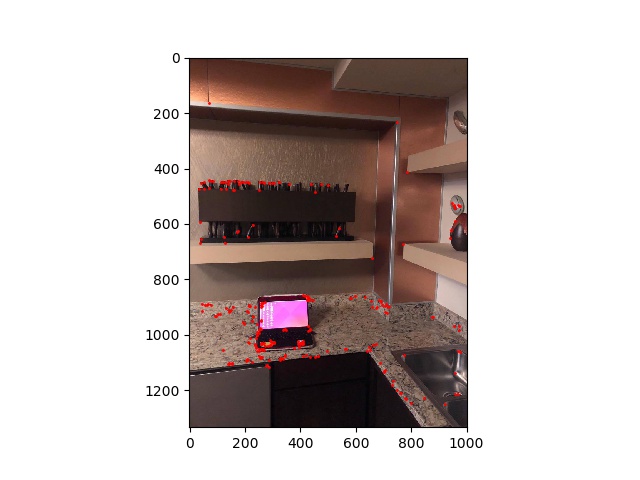
computer1 feature points

computer2 feature points

Part 5: RANSAC

To remove outliers left after the previous part, we need to use RANSAC to further fine tune the results. RANSAC first calculates a homography matrix by randomly selecting 4 correspondences. We use this homography matrix to warp all remaining points in image 1 to image 2, and count the inlier points. The inlier points are defined by using the dist2 function provided in the skeleton code to see if the warped point in image 1's distance to the corresponding point in image 2 is less than some epsilon. Epsilon is once again defined by the user. We calculate RANSAC many times, in this case 10000 times, to find the largest set of inlier points possible. We calculate our homography matrix using these sets of points and use it to do the final warp.

Results

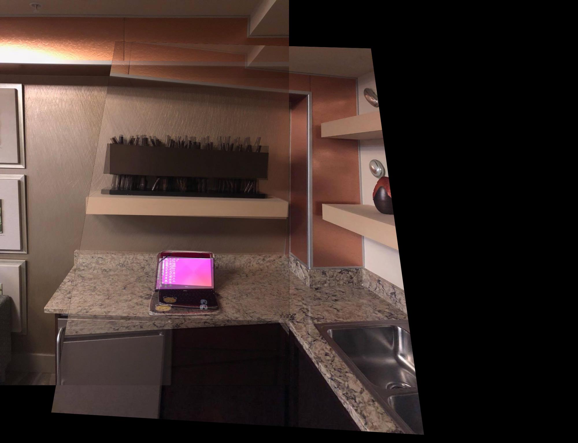
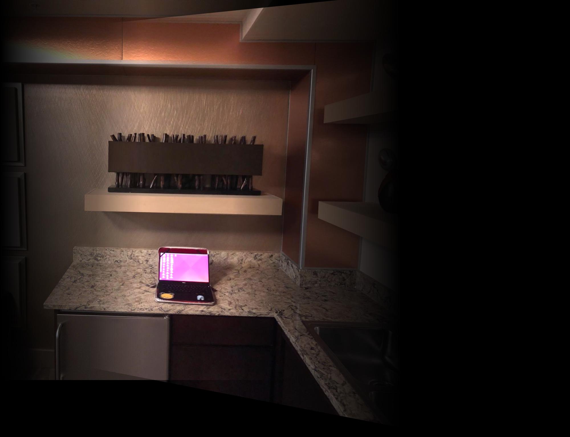
Manual	Auto
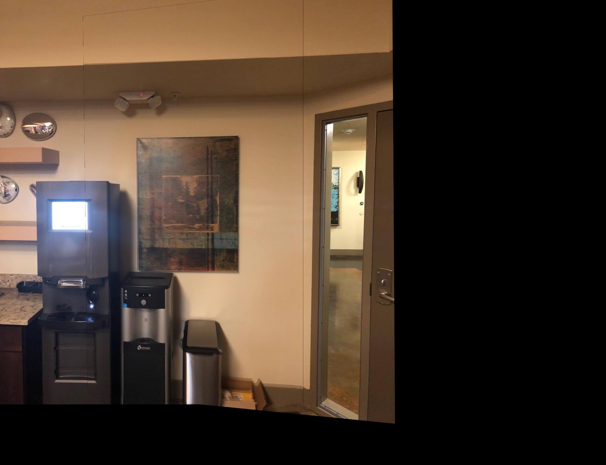
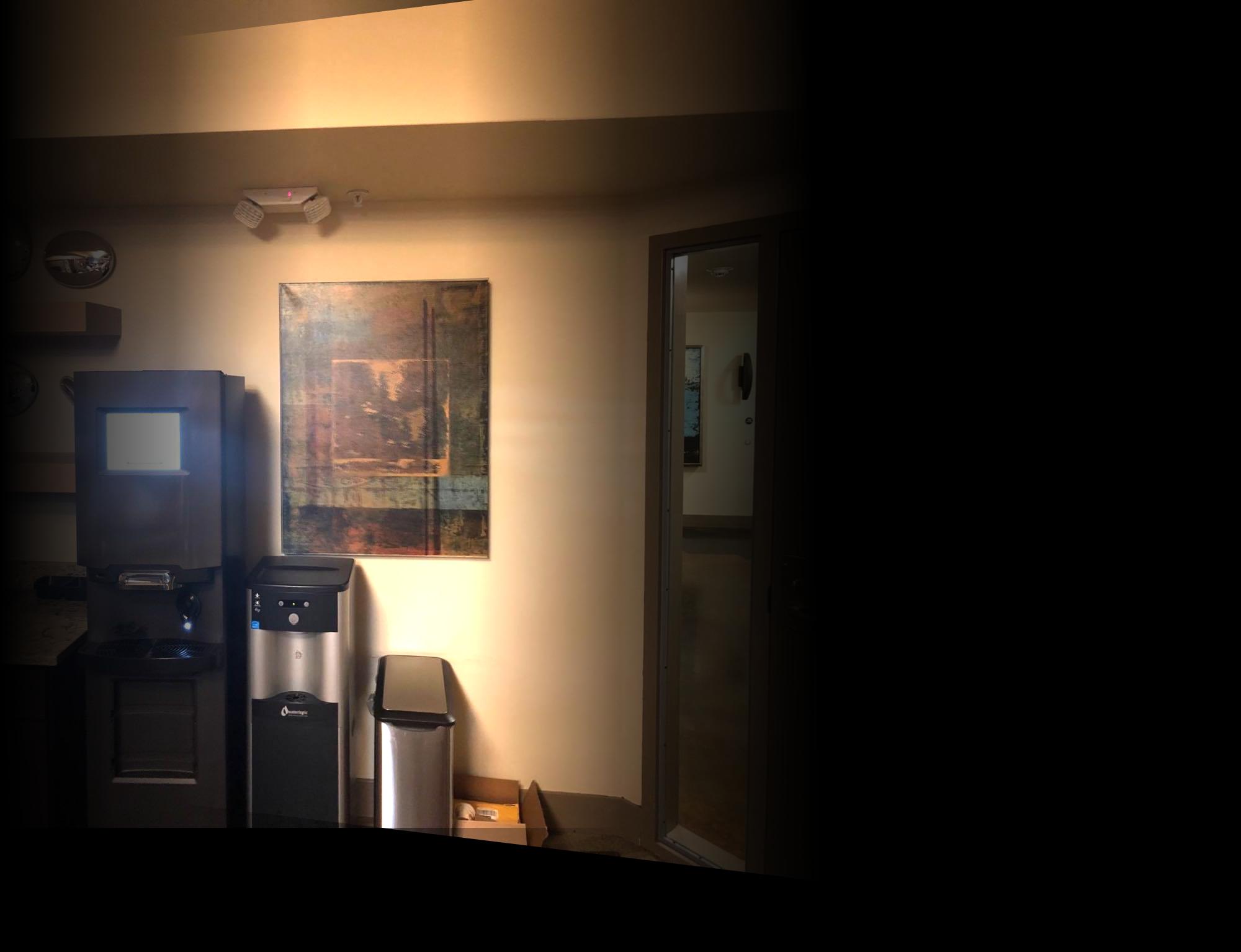
Manual	Auto
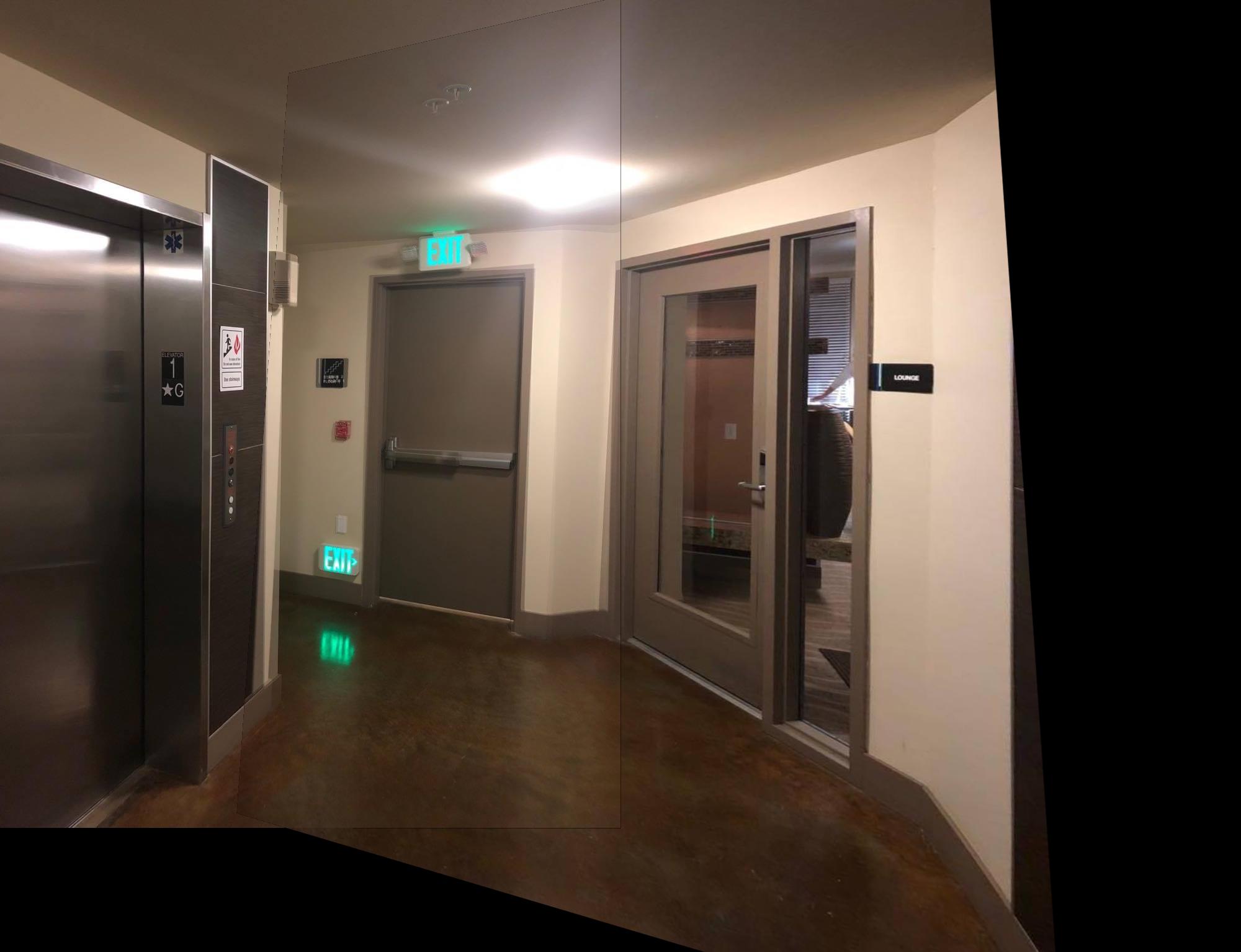
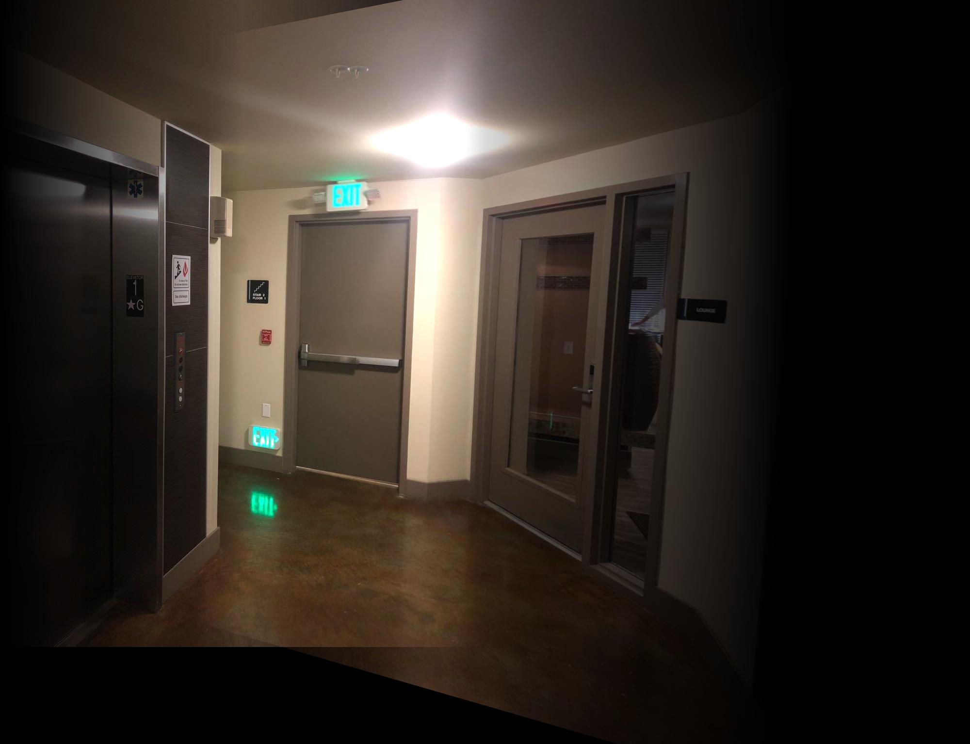
Manual	Auto

What I Learned

The coolest thing I learned was feature descriptors and feature matching. It's a very intuitive thought process which makes sense! You want to be able to describe your feature point in some way, so naturally, hashing the pixels make sense since you want some one-to-one correspondence. However, seeing it actually be used in a concrete way was very cool. Furthermore, the idea of hashing it in order to match it with another set of points was also really cool. Being able to automate this entire process of choosing correspondences was amazing as well.