CS194-26 Project 6: [Auto]stitching Photo Mosaics
cs194-26-afc, Kaiwen Zhou
-
Part A: Image Warping and Mosaicing
-
Part B: Feature Matching for Autostitching
Part A: Image Warping and Mosaicing
In this project, we're exploring a form of image warping with an interesting application - image mosaicing. We take several photographs and create an image mosaic by registering, projective warping, resampling, and compositing them. Central to this project is computing homographies and using them to warp images.
Shooting Photos
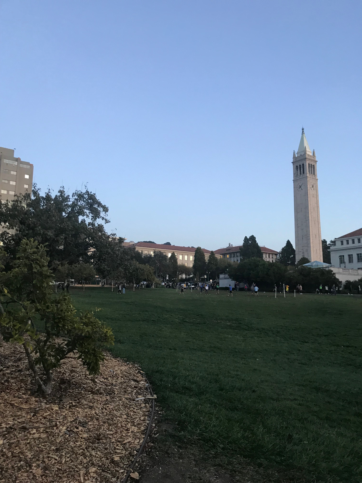
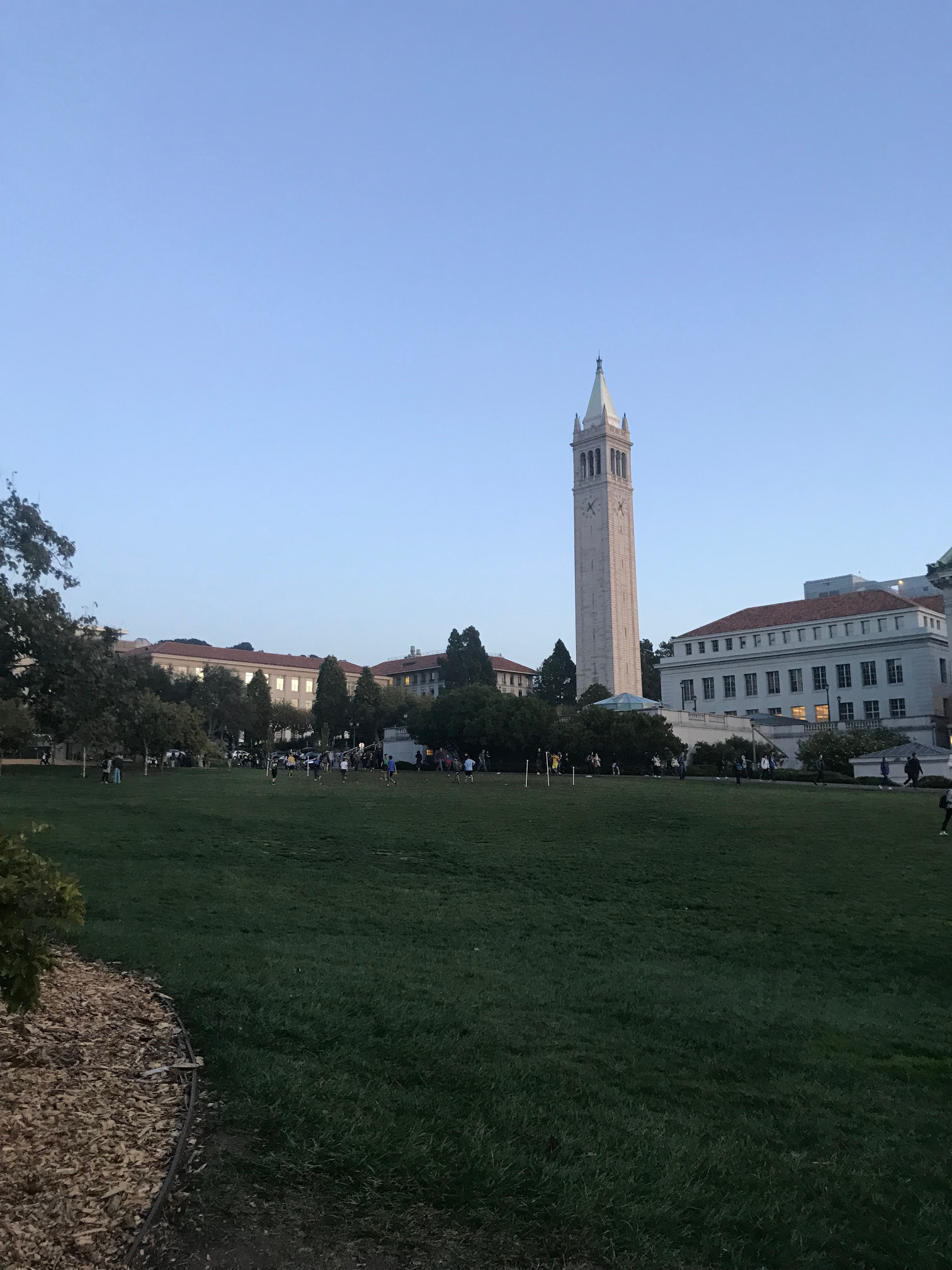
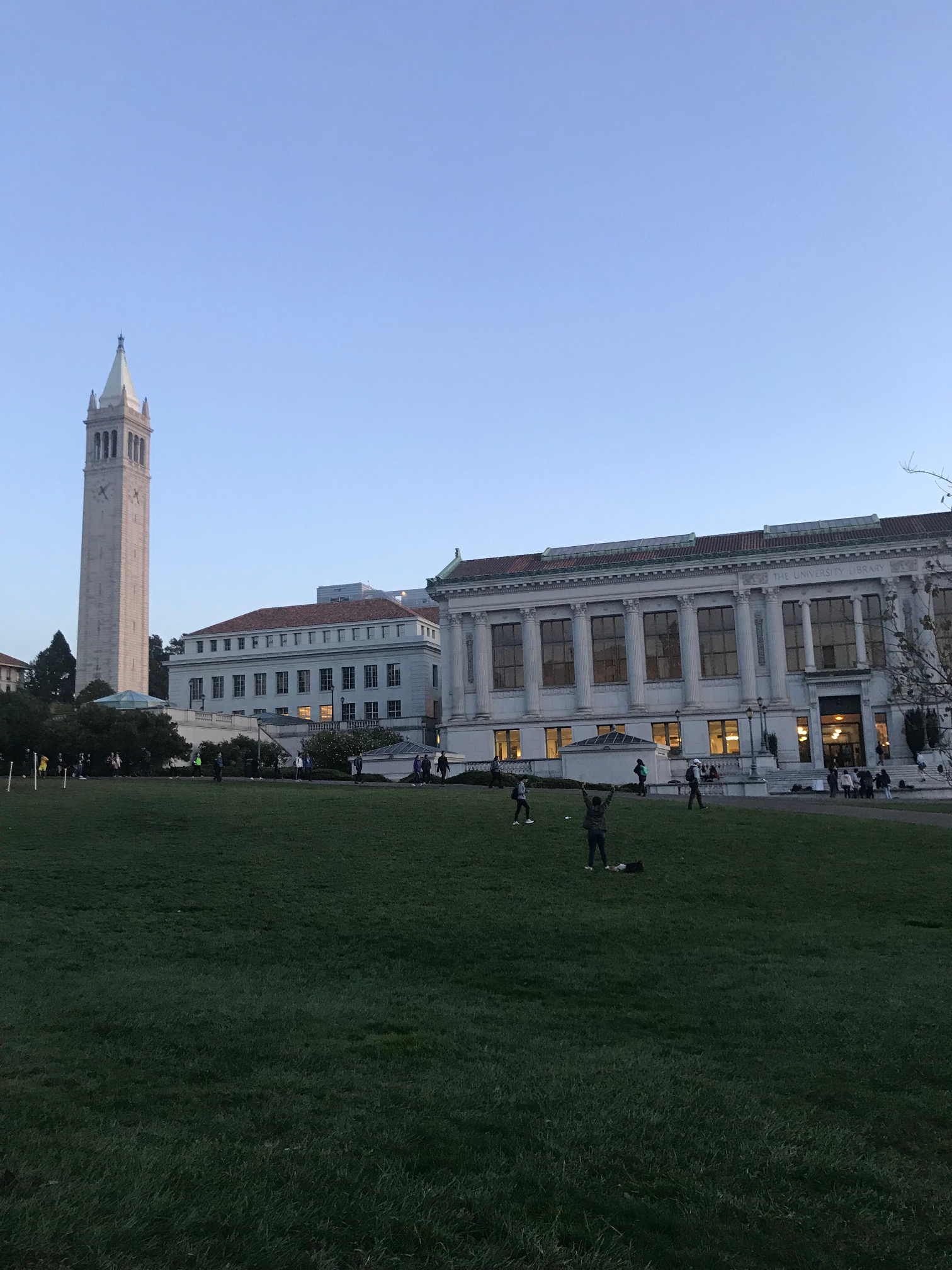
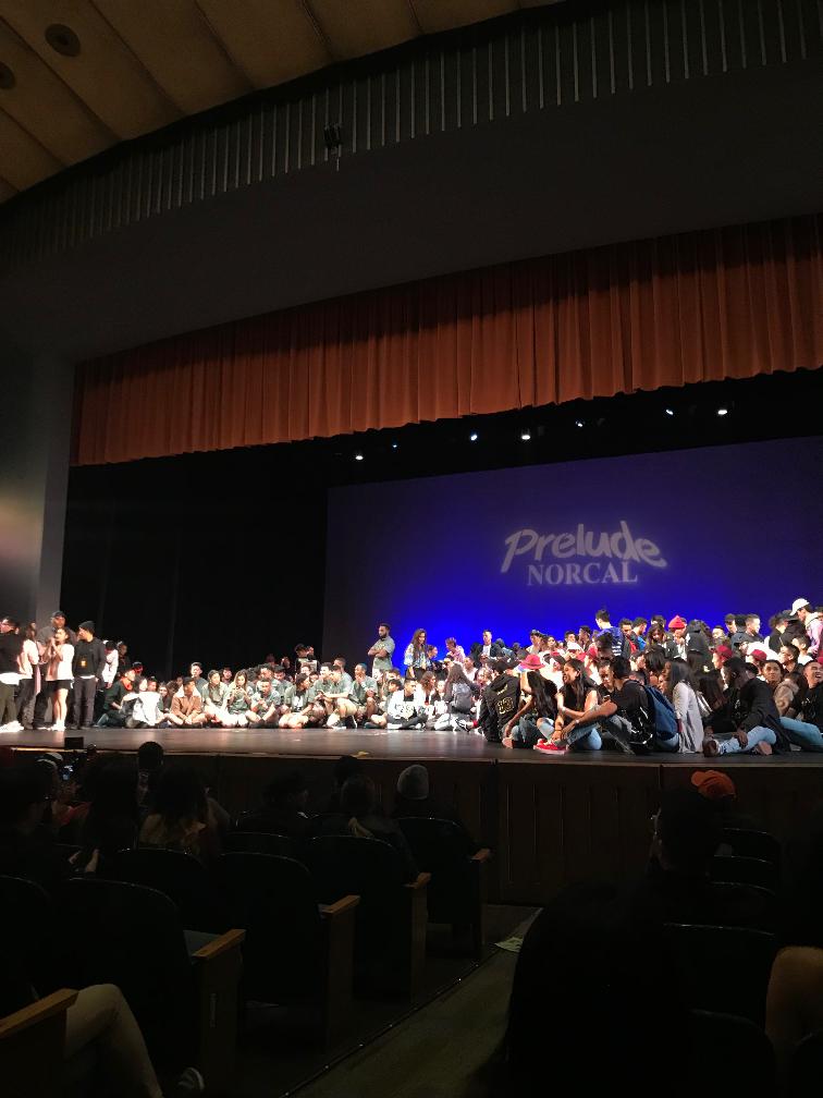
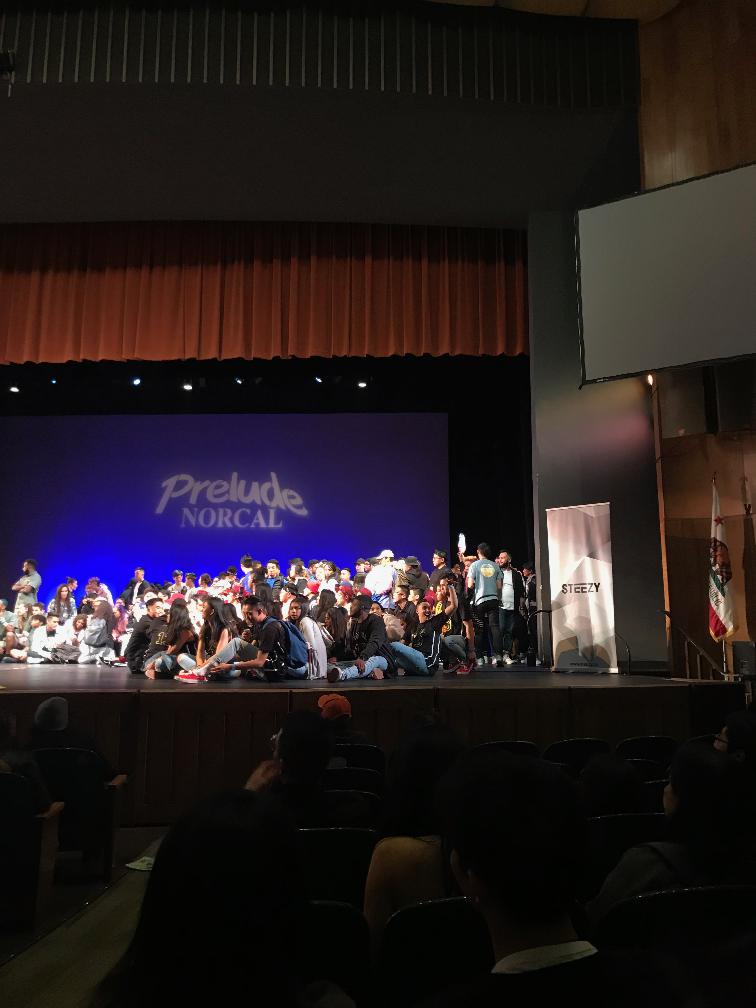
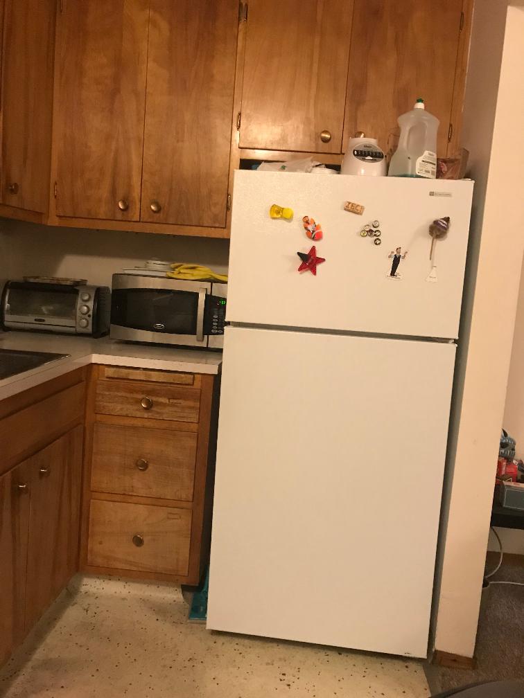
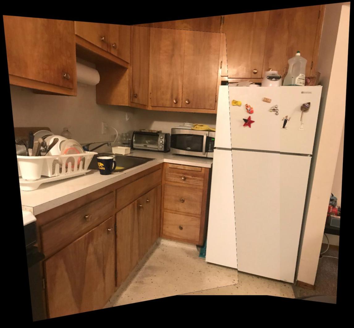
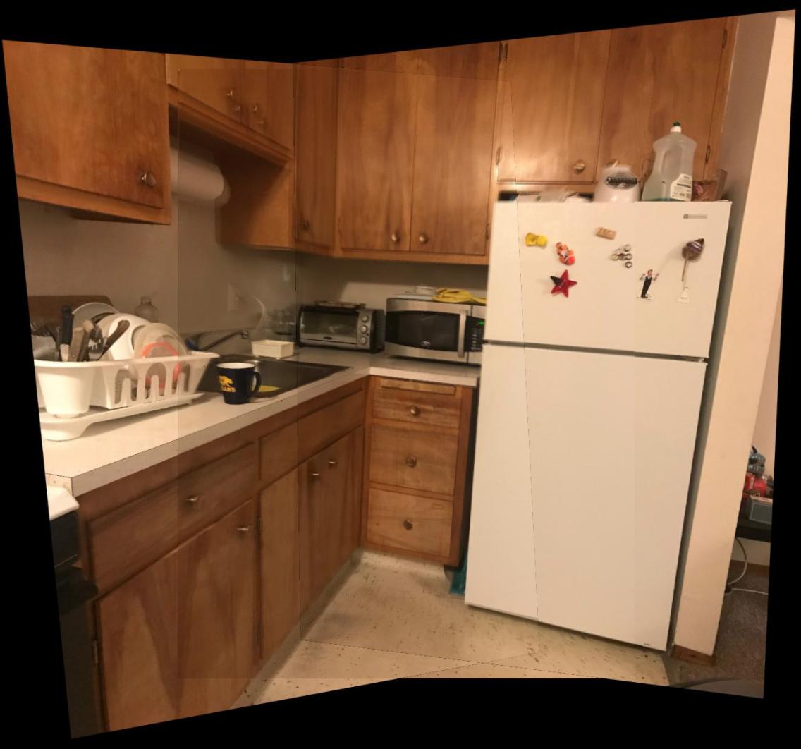
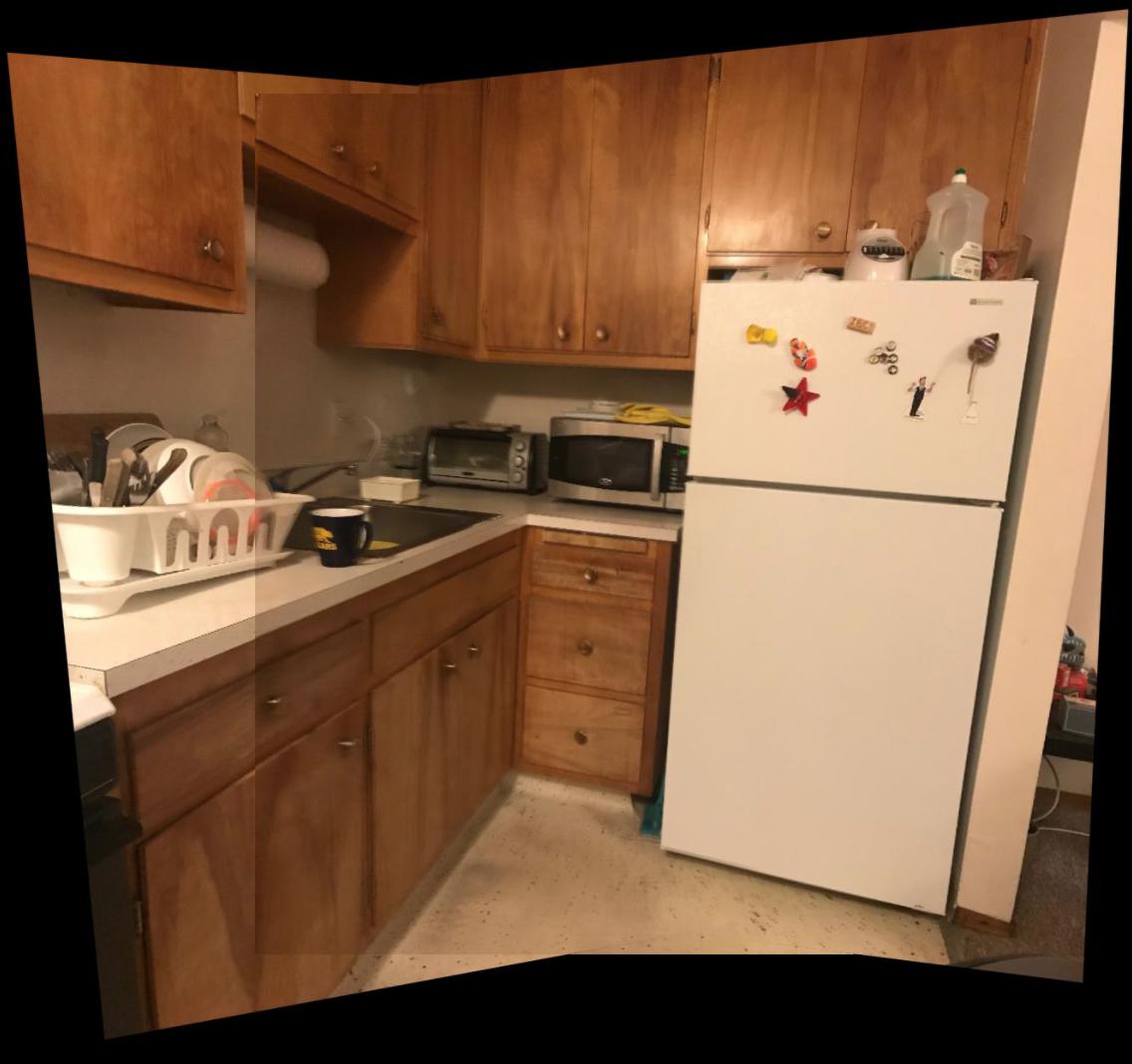
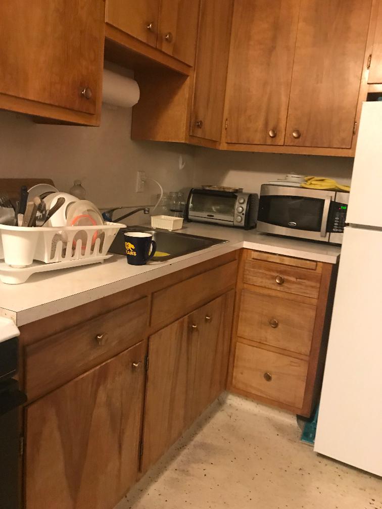
Unfortunately, I don't have a digital camera or a tripod. Instead, I managed to take a series of vertical images using my iPhone by rotating it while holding it in place. The locations I chose included Memorial Glade, my friend's kitchen, and a dance competition (outside of Berkeley).
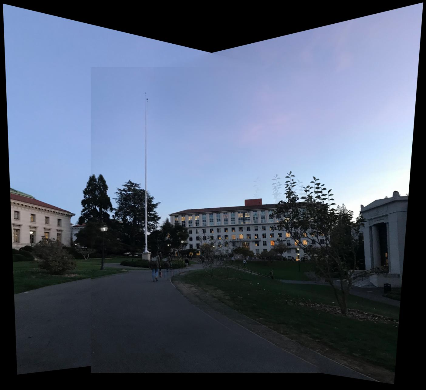
Memorial Glade
Prelude
My Friend's Kitchen
Recovering Homographies
In order to rectify and warp images, we first have to recover the transformation parameters between each pair of images. In this case, our transformation is a homography H in the form p’=Hp, where H is a 3x3 matrix with 8 degrees of freedom. One way to recover the homography is via a set of (p’,p) pairs of corresponding points taken from the two images.
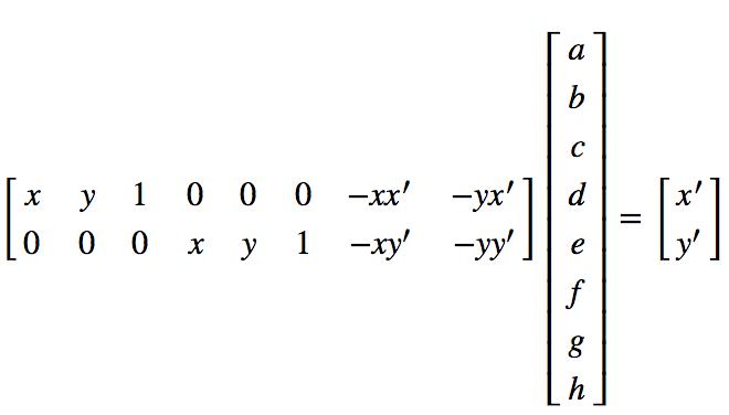
I used ginput to select point correspondences between images. Because our system is overdetermined, we can't solve directly for the matrix H - I instead solved for the explicit formulas for each variable in H, and set up a least squares equation to solve for the variables themselves.
After some math, the least squares equation amounted to:
Image Rectification
As a preliminary test of our warping function, we perform a simple rectification of an aspect of an image into a rectangular shape. For my rectification examples, I chose my mac keyboard & a photo of the campanile.
Mac Keyboard
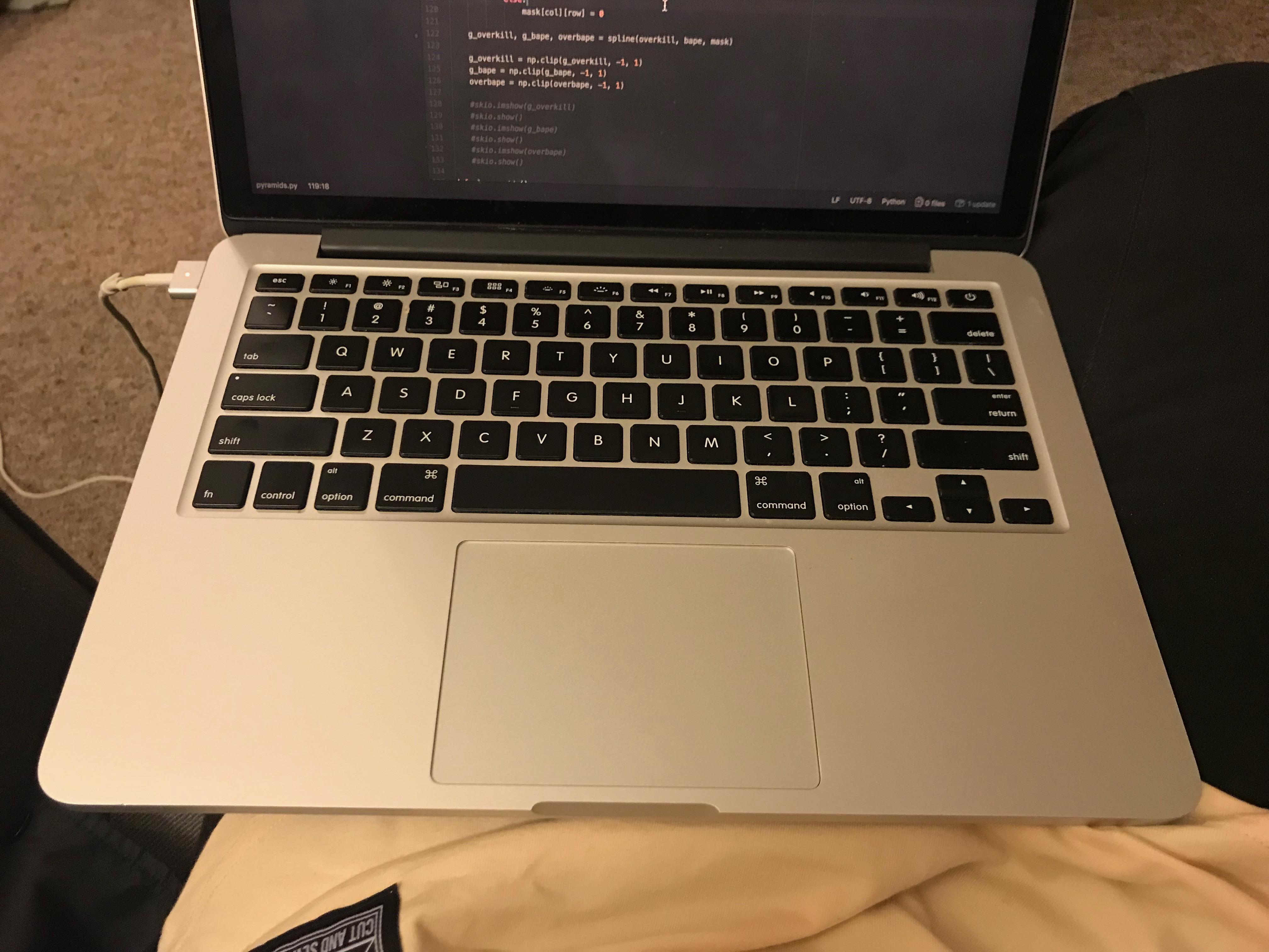 original
|
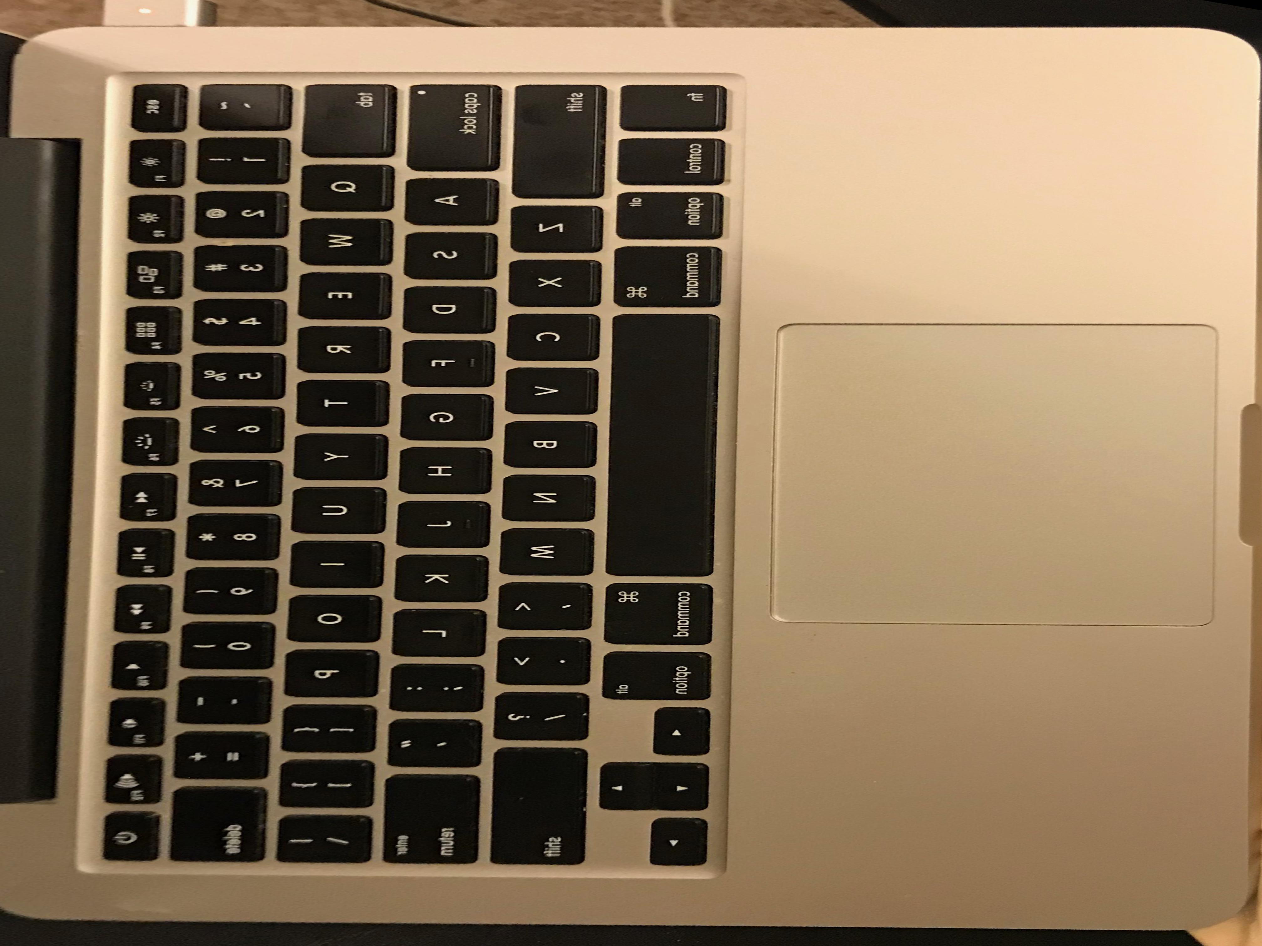 rectified
|
Campanile
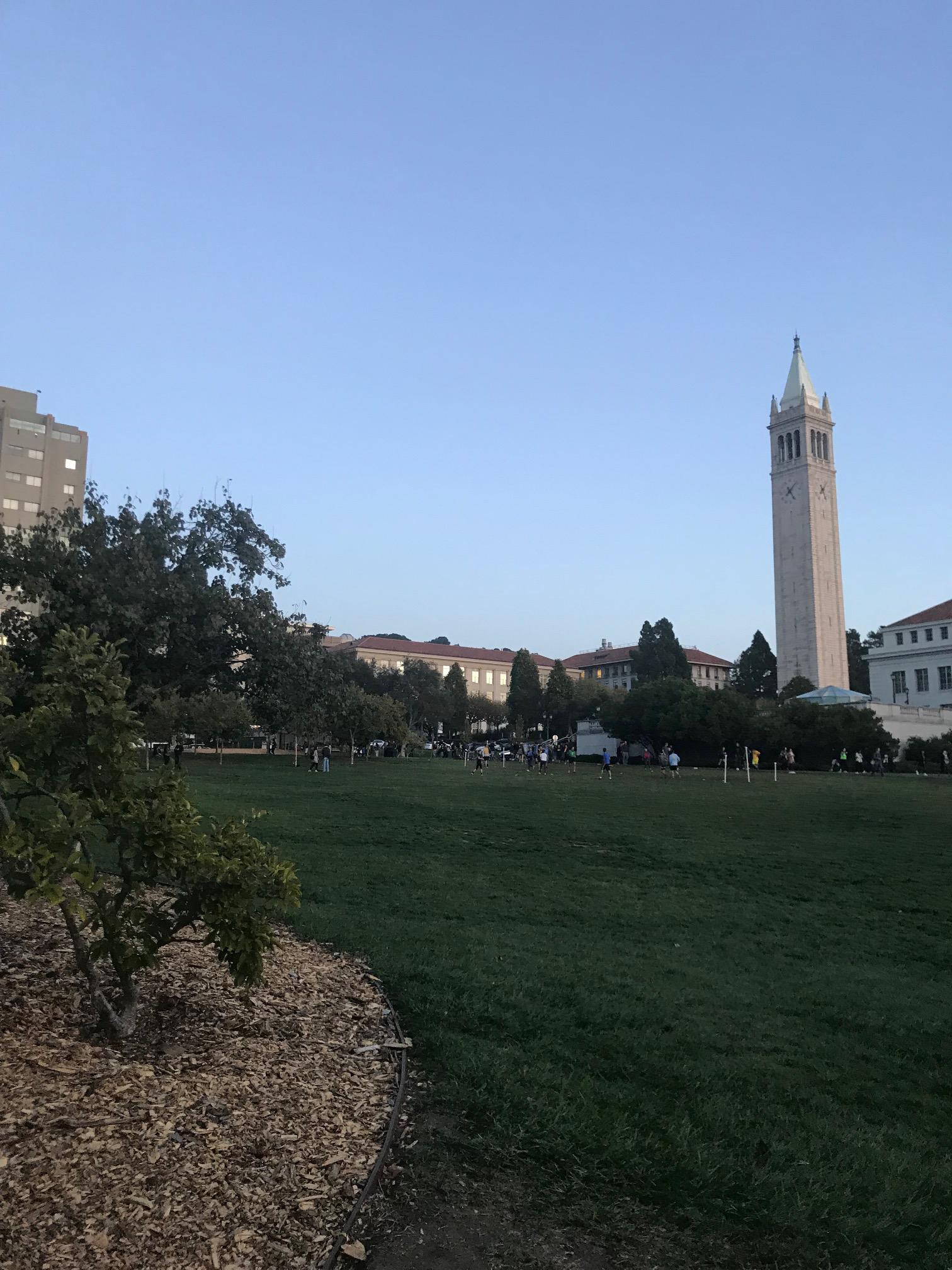 original
|
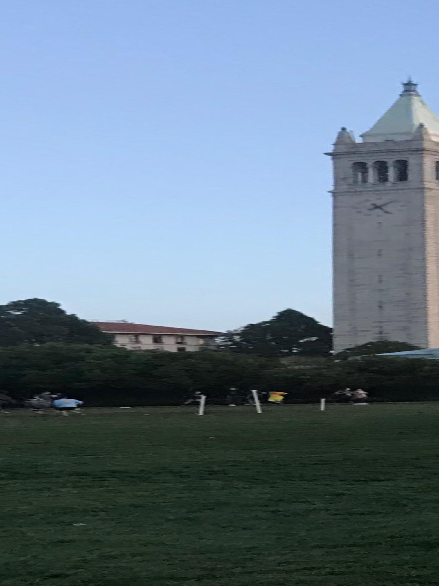 rectified
|
Final Mosaics
For my results, I performed three different types of blending. The first was simple overlap blending in which I only showed another image in black areas of the original image. I also performed a simple weighted blend in which the overlap consisted of half one image and half the other. Lastly, I performed linear blending by weighing each pixel by the distance from each image center. Overall, linear blending gave the best results.
My campanile/memorial glade image blended the best because much of it consisted of blue sky, with few high frequency objects to blend. The campanile is a bit blurry in linear blending, because the aligning is a little bit off.
Campanile
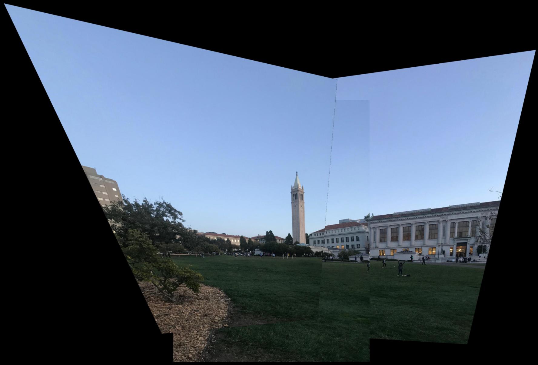 simple blend
|
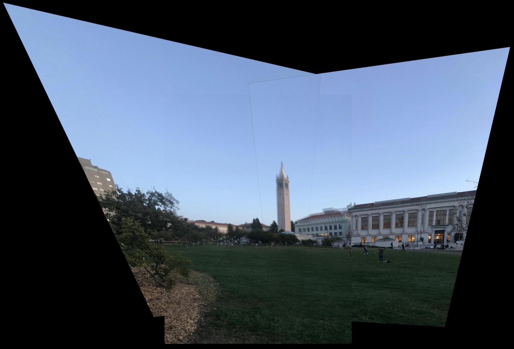 weighted blend
|
 linear blend
|
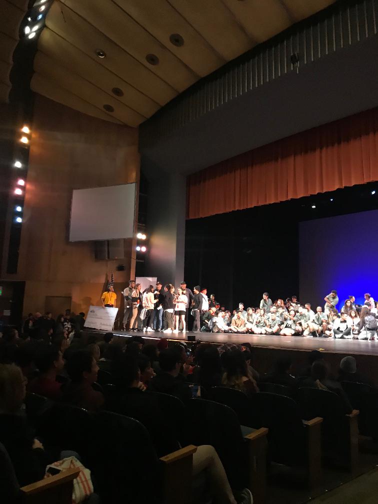
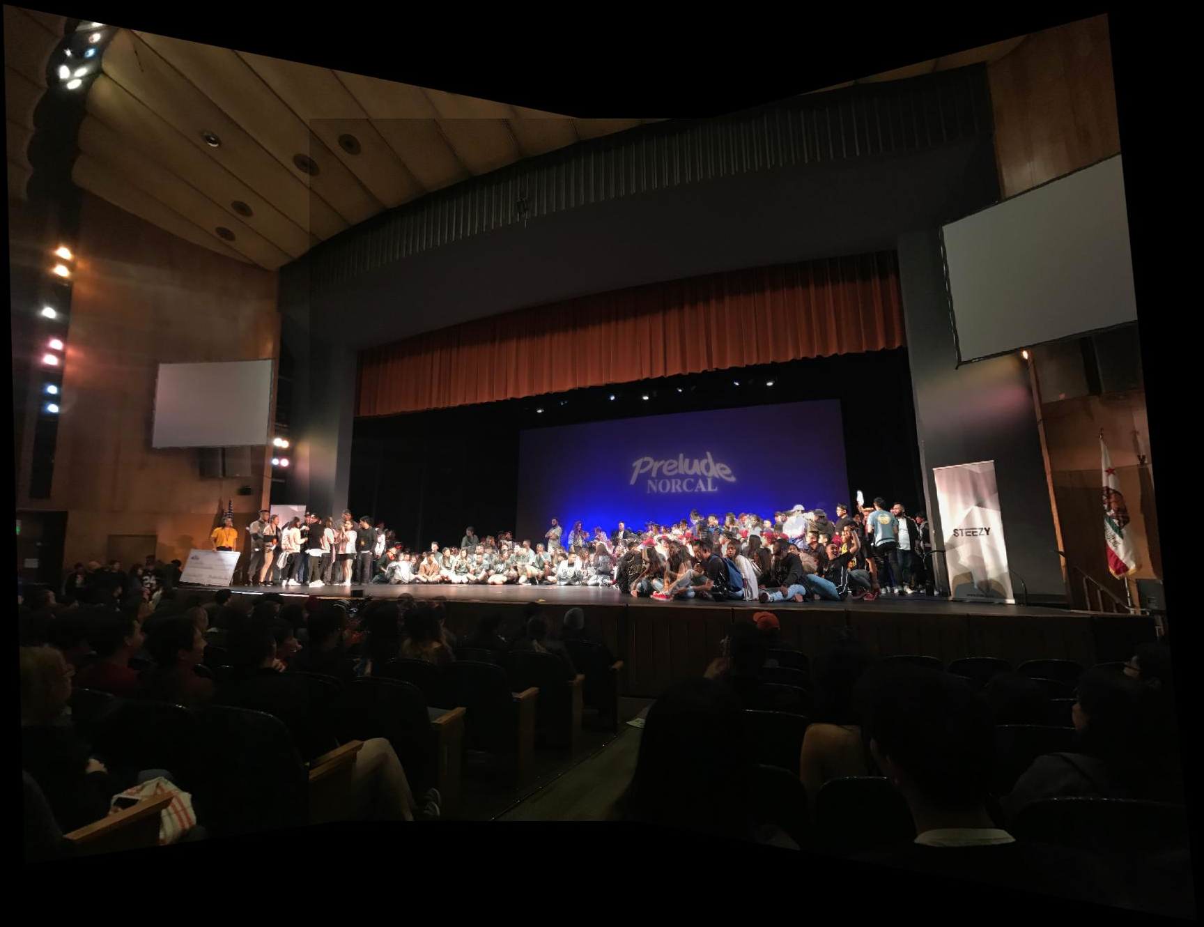
Prelude
Instead of working on my project on Saturday night, I instead went to a dance competition. While I was there, I decided I might as well take photos for my panorama. The panoramas didn't blend too well, but that was to be expected - my iPhone camera lighting was automatic & was thrown off by the indoor lighting. In addition, people slightly shifted resulting in artifacts in the blended panorama.
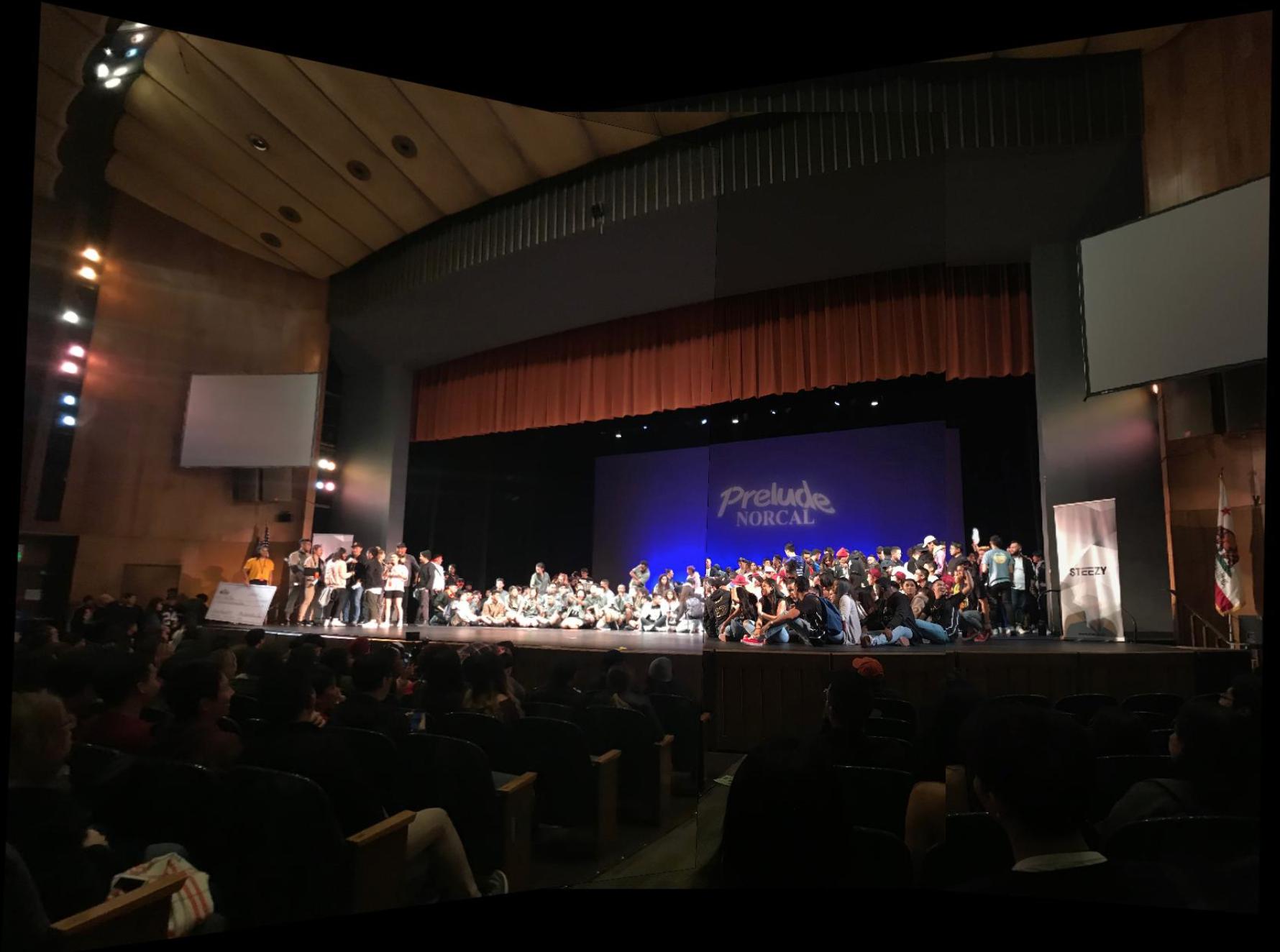 simple blend
|
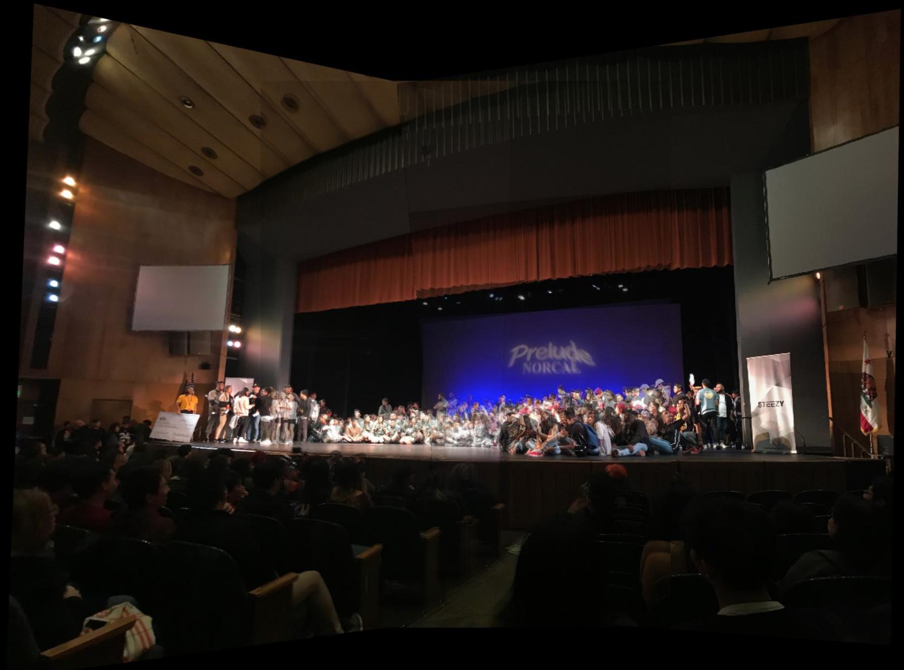 weighted blend
|
 linear blend
|
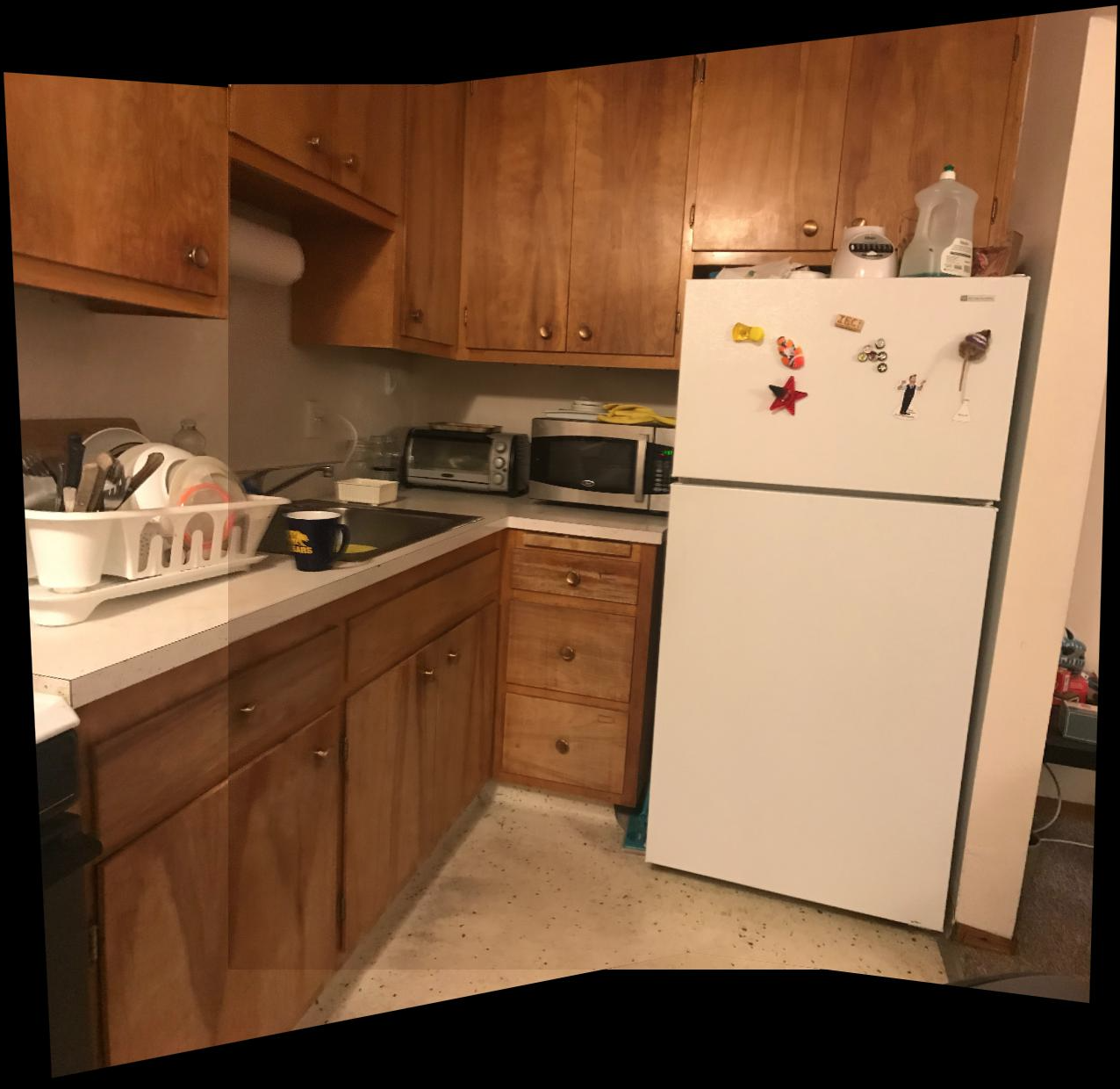
The kitchen also gave pretty respectable results, as much of the blending lines were on mono-colored objects and there were few details to cause artifacts for the blended images.
Kitchen
 simple blend
|
 weighted blend
|
 linear blend
|
What I learned (part A)
It's really cool to see the types of transformations that matrices can perform on images! Being able to warp the perspectives of an image seems like a very powerful tool to post-process images after they've been taken.
Part B: Feature Matching for Autostitching
In order to demonstrate my approach for feature matching, I will be using the sample images of the kitchen from part A.
Kitchen
 im1
im1
|
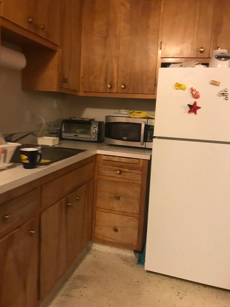 im2
im2
|
Detecting corner features in an image and Adaptive Non-Maximal Suppression
I used the python starter code in harris.py to detect Harris interest Points. Harris interest points are measured by their corner response, so the higher the response at a point, the stronger of a Harris corner it is.
Afterwards, I followed the approach in the paper to implement adaptive non-maximal suppression. This step is important because it limits the total number of interest points to consider while ensuring that we keep our strongest Harris points of interest. It does this by evenly distributing strong points across the entire image. The main idea is for all Harris points $\mathbf{x_i}$ we find the minimum suppression radius through the given formula
$$r_i = \min_{j} |\mathbf{x_i} - \mathbf{x_j}|, s.t. f(\mathbf{x_i}) < c_{robust}f(\mathbf{x_j}) $$
where $\mathbf{x_j}$ is another Harris point, $f$ is the function that will return a given points corner response, and $c_{robust} = 0.9$ is a constant used to assure that $f(\mathbf{x_i})$ needs to be significantly smaller than $c_{robust}f(\mathbf{x_j}) $ in order for $x_j$ to affect $r_i$. Essentially, we assign a radius $r_i$ to each point that's equal to the distance of the closest "significantly greater" point. Intuitively, for smaller values of $r_i$, then $\mathbf{x_i}$ has a small corner response in respect to its close neighbors. For bigger values of $r_i$, $\mathbf{x_i}$ has a stronger corner response than those of its neighbors. Thus, Harris points with larger $r_i$ are the "strongest" Harris points in their respective areas of the image. I chose to keep the $\mathbf{x_i}$ corresponding to the 200 largest $r_i$, which leads to spacially well distributed Harris points.
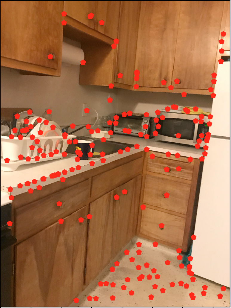 im1 corners
|
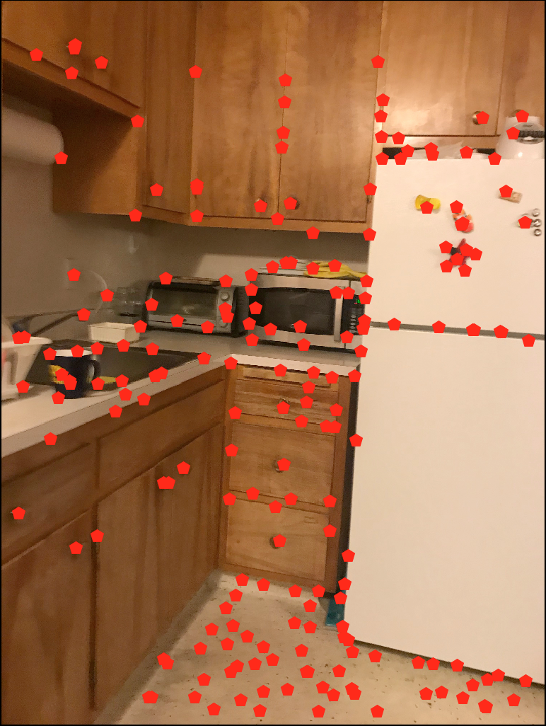 im2 corners
|
Feature Descriptors
For each of the points kept from the previous part, I found a corresponding feature descriptor of the pixels surrounding the point. I used the descriptor described in the MOPS paper, which consisted of a 40x40 patch surrounding for a given Harris interest point. Then I used imresize, which blurred the image with a Gaussian and downsized it into an 8x8 patch, then subtracted the mean and divided by the standard deviation (bias/gain normalization). By doing this, we obtain a descriptor that contains the low frequencies at the point and its local surroundings and deals with changes in color intensity through normalization.
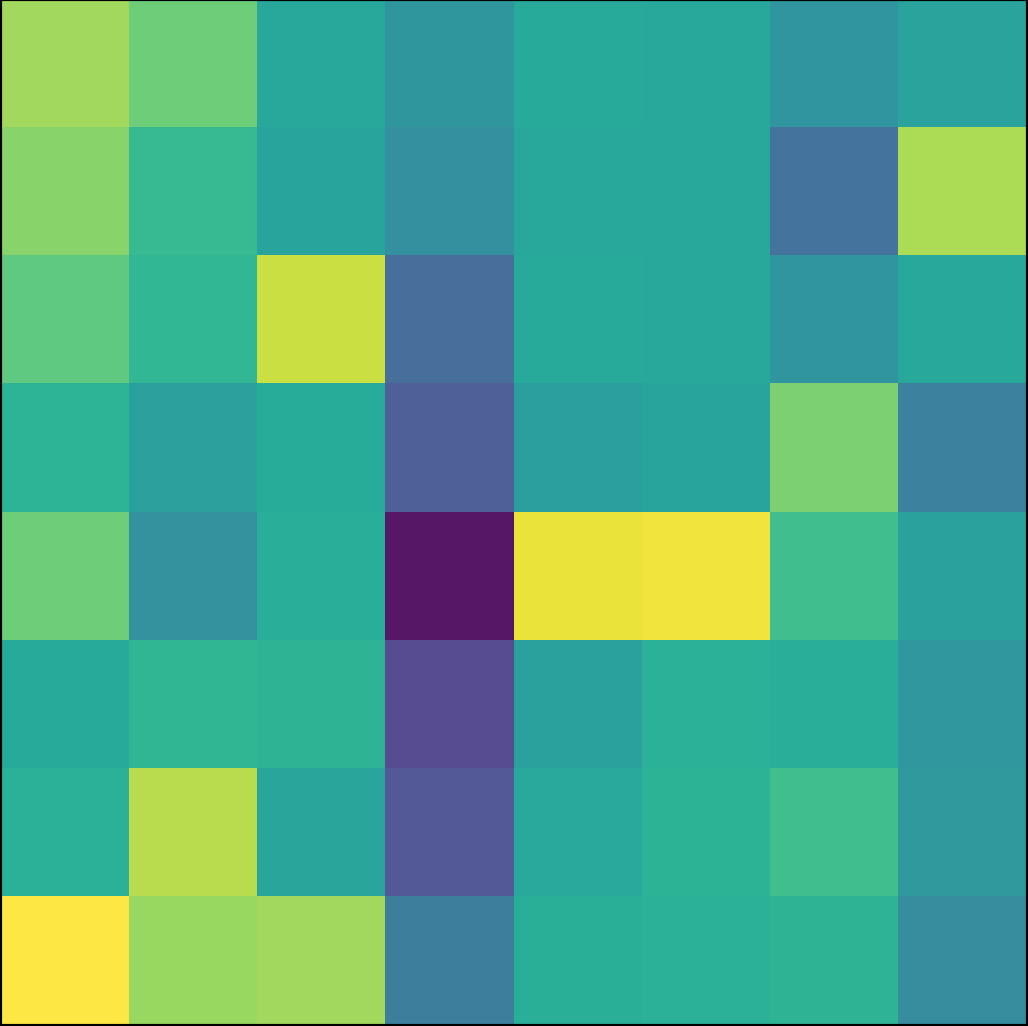 example im1 feature
|
 example im2 feature
|
Feature Matching
To match the Harris points between two images, I used a Sum of Squared Differences elementwise between points on the feature descriptors between each image. I used the Lowe algorithm mentioned in the paper which found the SSD of the best match and the SSD of the second best match (1-NN and 2-NN) respectively. I then thresholded based on the ratio 1-NN/2-NN. We want to choose points that minimize this ratio - lower ratios mean that there's only one definite "best" match that we have to consider, while higher ratios signal a higher degree of confusion between features. Thus, I chose to keep matches with the ratio below 0.5. My results from this section are below.
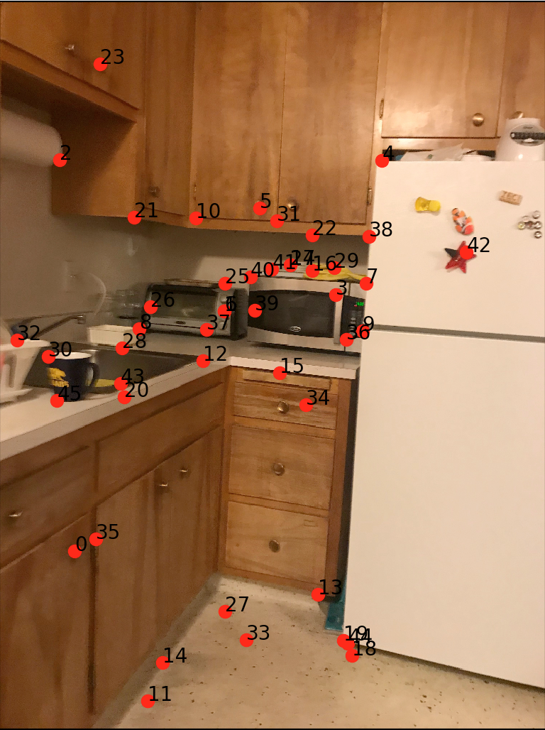 Matches in im1 (labeled by #)
|
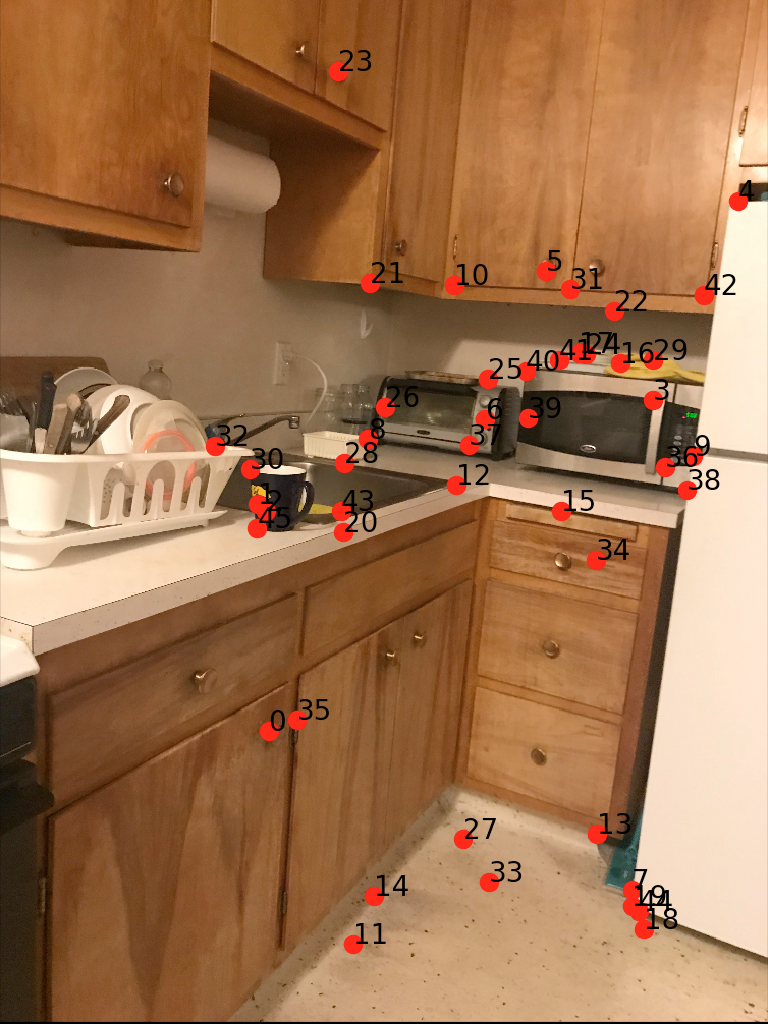 Corresponding matches in im2 (labeled by #)
|
Random Sample Consensus (RANSAC)
With the point correspondences in place due to the feature matching, the only thing left to do before stitching is to the compute the homography between the images. However, there still may be outlier points (false matches) in the point correspondence given by the feature matching.
Thus, I used the RANSAC algorithm. I took a sample of 4 random matchings, used them to compute a homography, and applied the projective transform to each matching I had using SSD. I thresholded on matchings with an SSD less than 50 for an optimal transform, which I kept as inliers. I would keep a running count of the maximum number of inliers for each case, which I updated each time I ran RANSAC. When that was done, I took the inliers for the maximum case & used them to compute my final homography for the image stitch.
Final autostitched results!
All results here were blended using linear blending.
Prelude
 Automatic stitching
|
Manual stitching
|
Autostitching definitely aligned better and seemed to fix some ghosting problems I had originally (because of all the detail within the people in the panorama).
Kitchen
 Automatic stitching
|
Manual stitching
|
I took some new images to create mosaics with after finishing part A.
Museum of Ice Cream
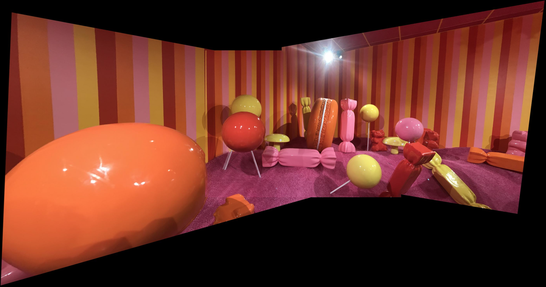 Automatic stitching
|
Dwinelle
 Automatic stitching
|
Summary
This is probably one of my favorite projects result-wise (besides the countless hours spent debugging)! I was surprised at how easily autostitching found correspondence points & how nice the results looked, especially considering how much of a pain manual point correspondence was.