Part A: Overview
The purpose of the first part of the project was to get experience with image warping. Our end result of this part of the project was to create a mosaic. To do so, we shot and digitalized pictures, recovered homographies, warped the images, and then blended the images into a mosaic.Part 1
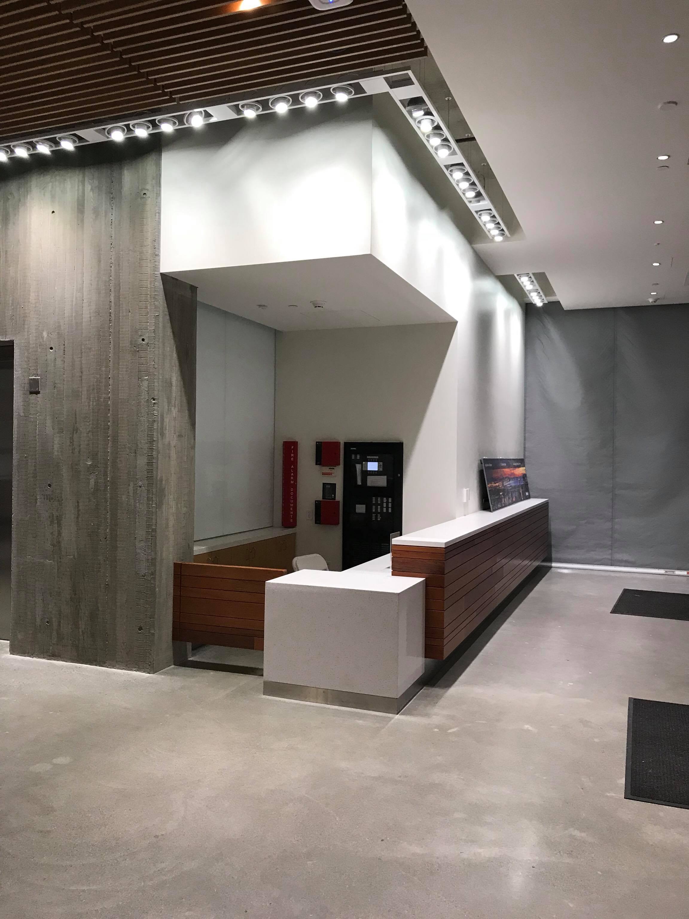
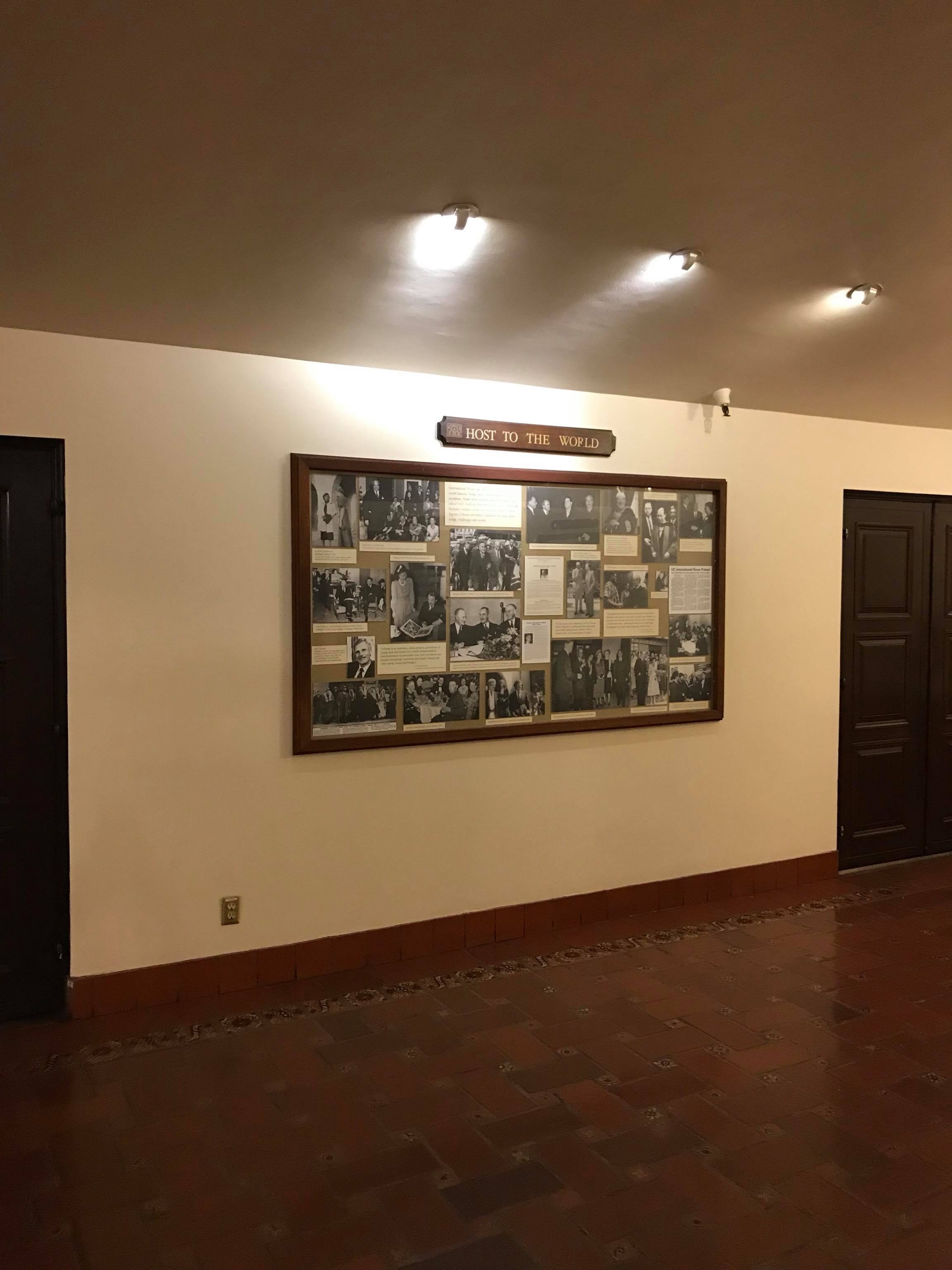
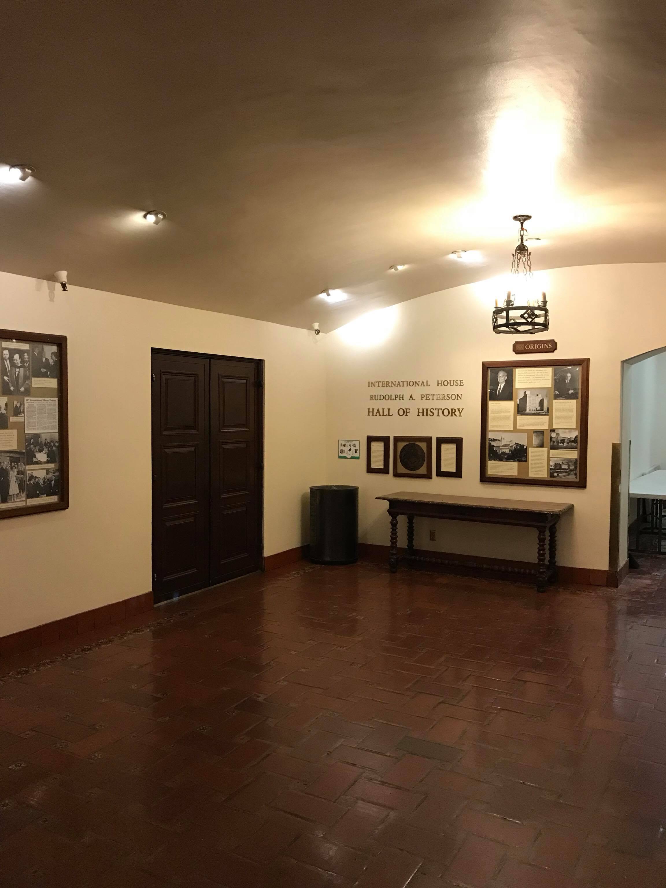
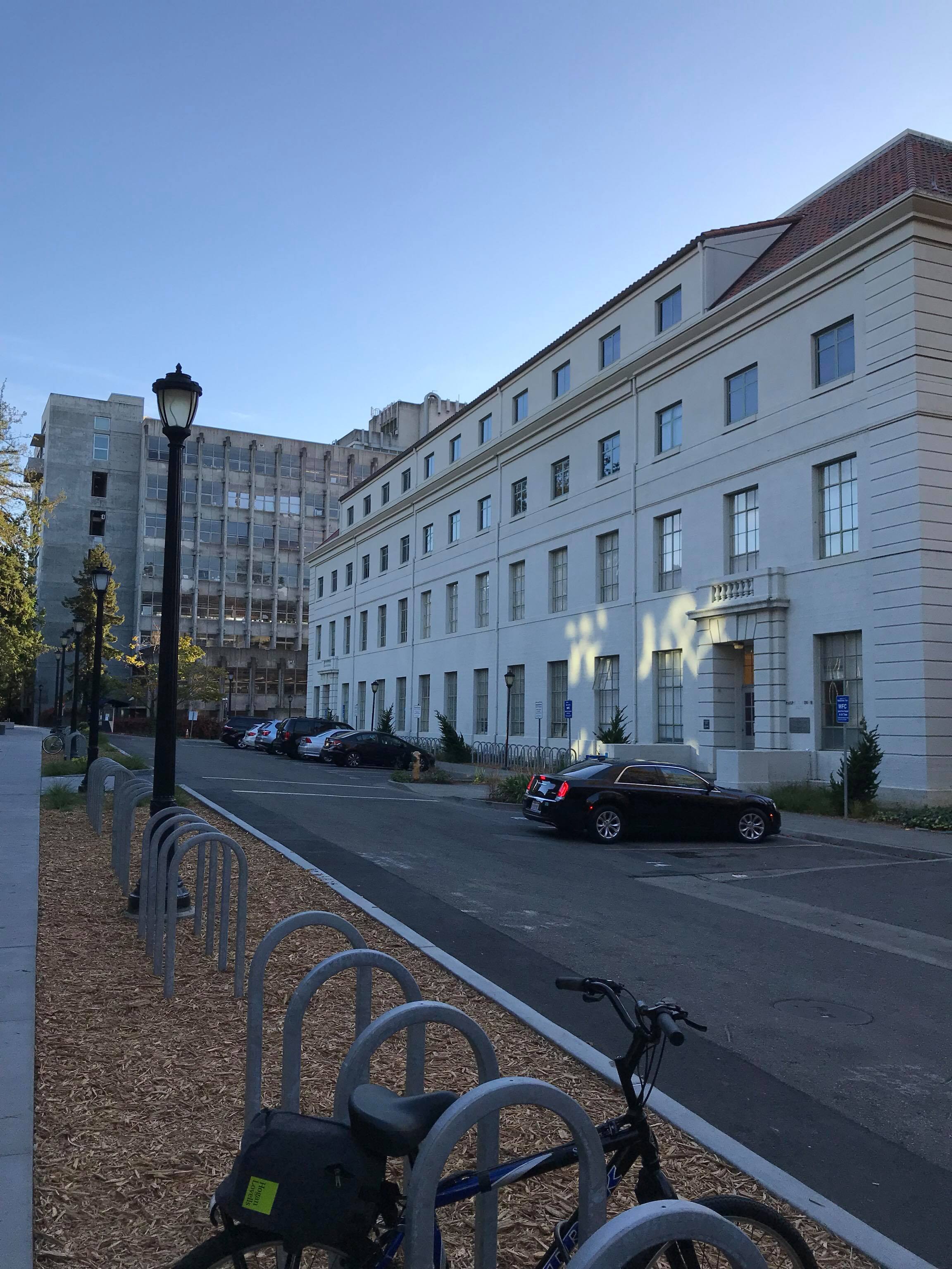
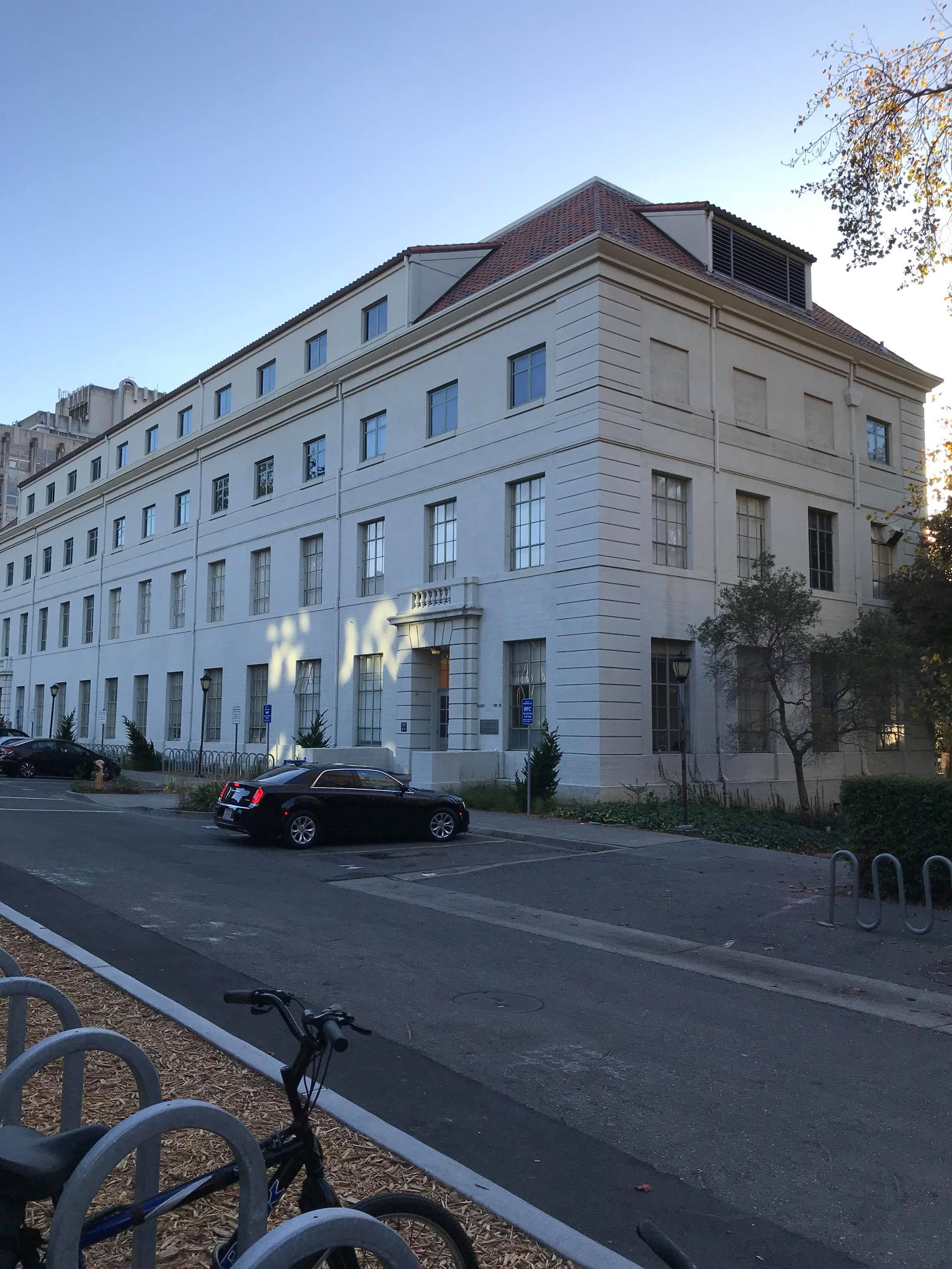
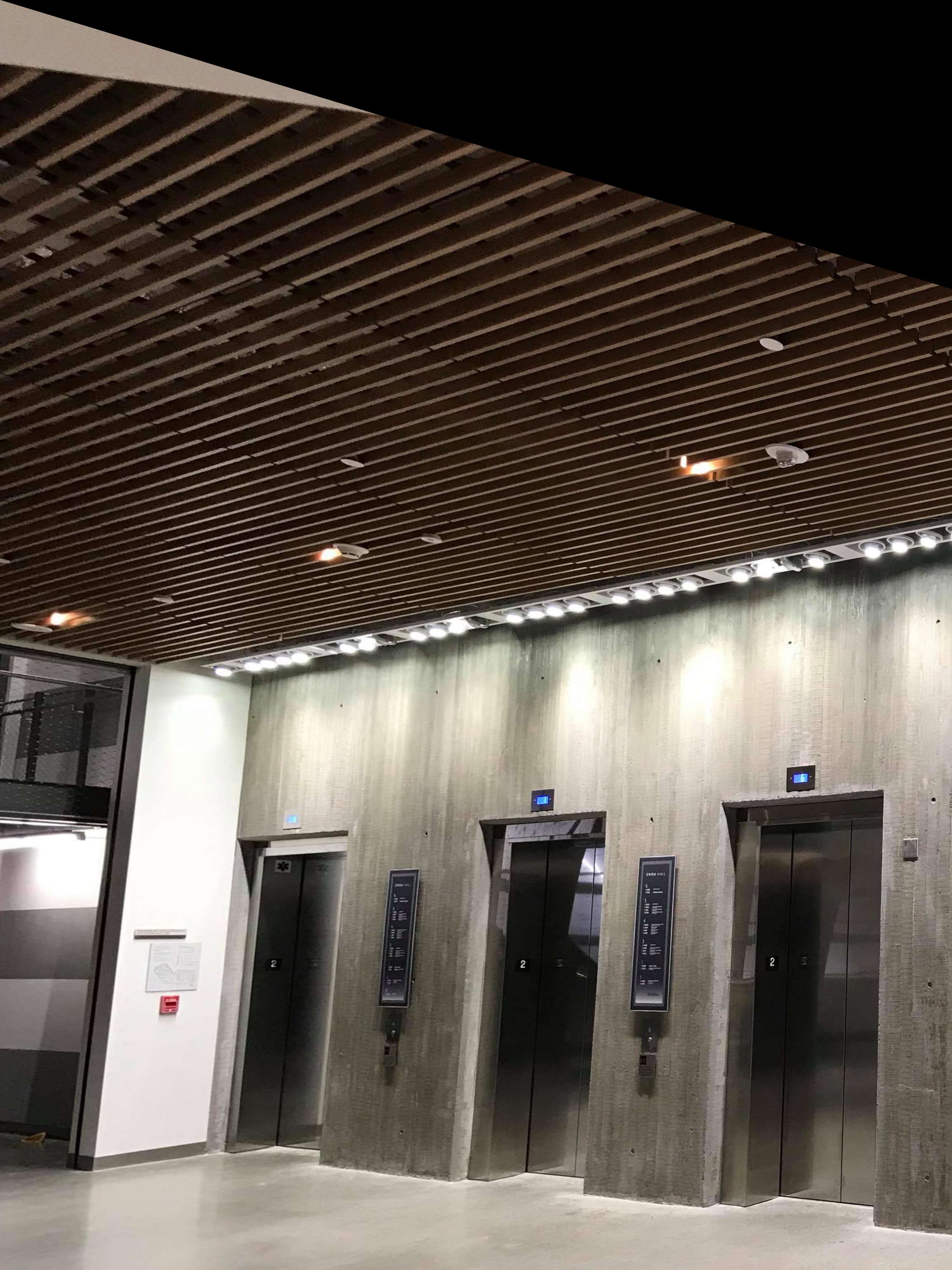
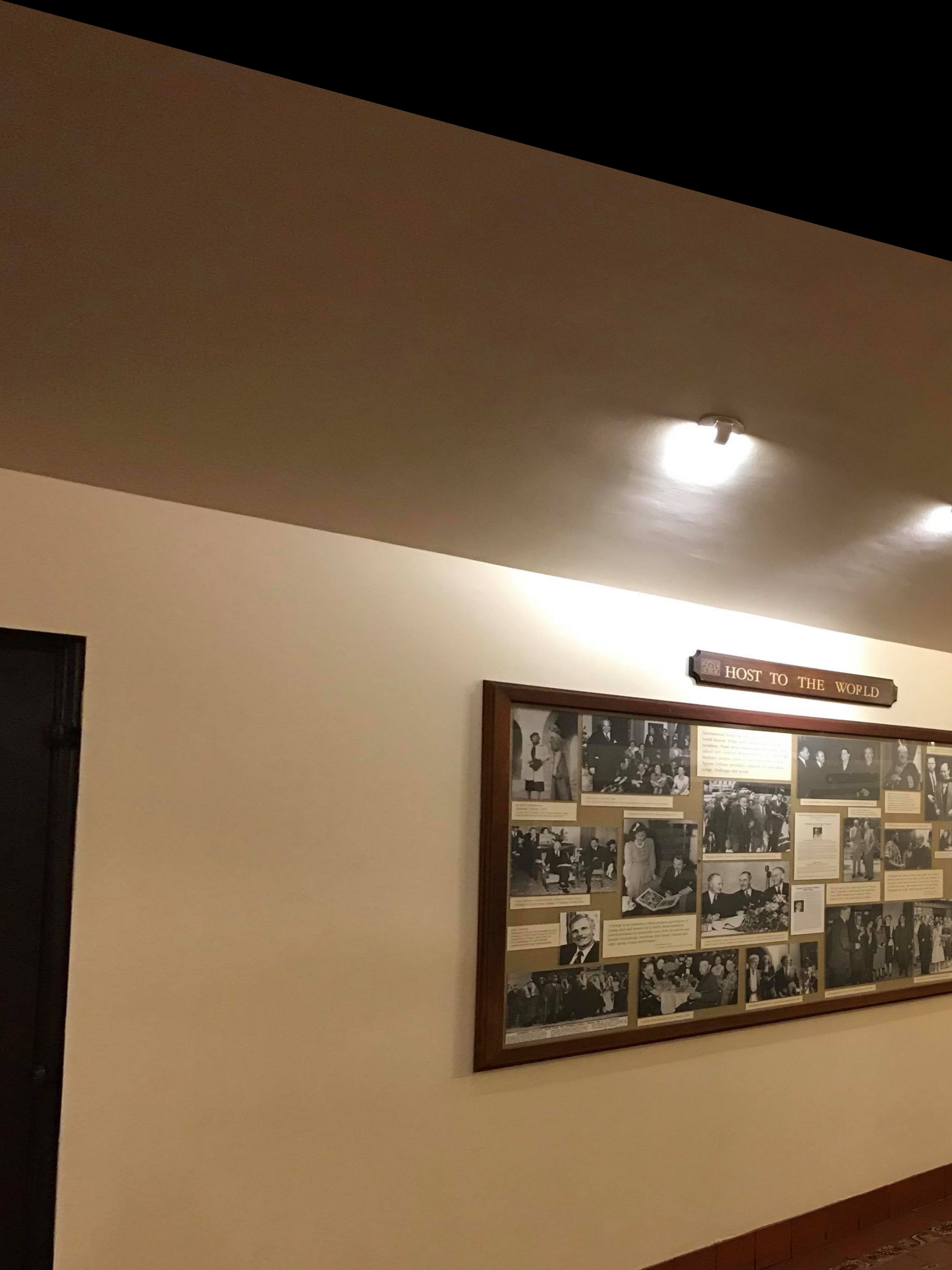
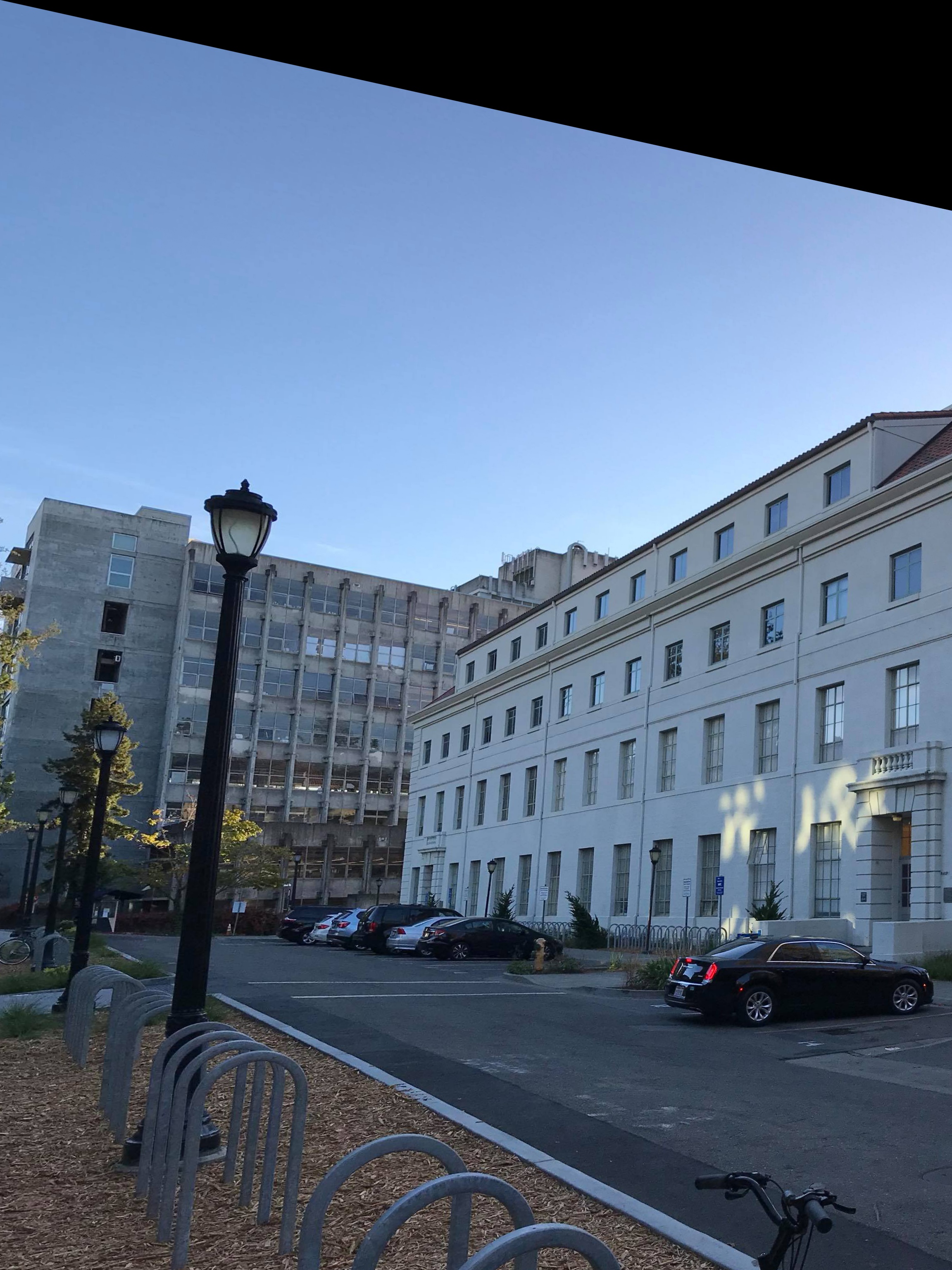
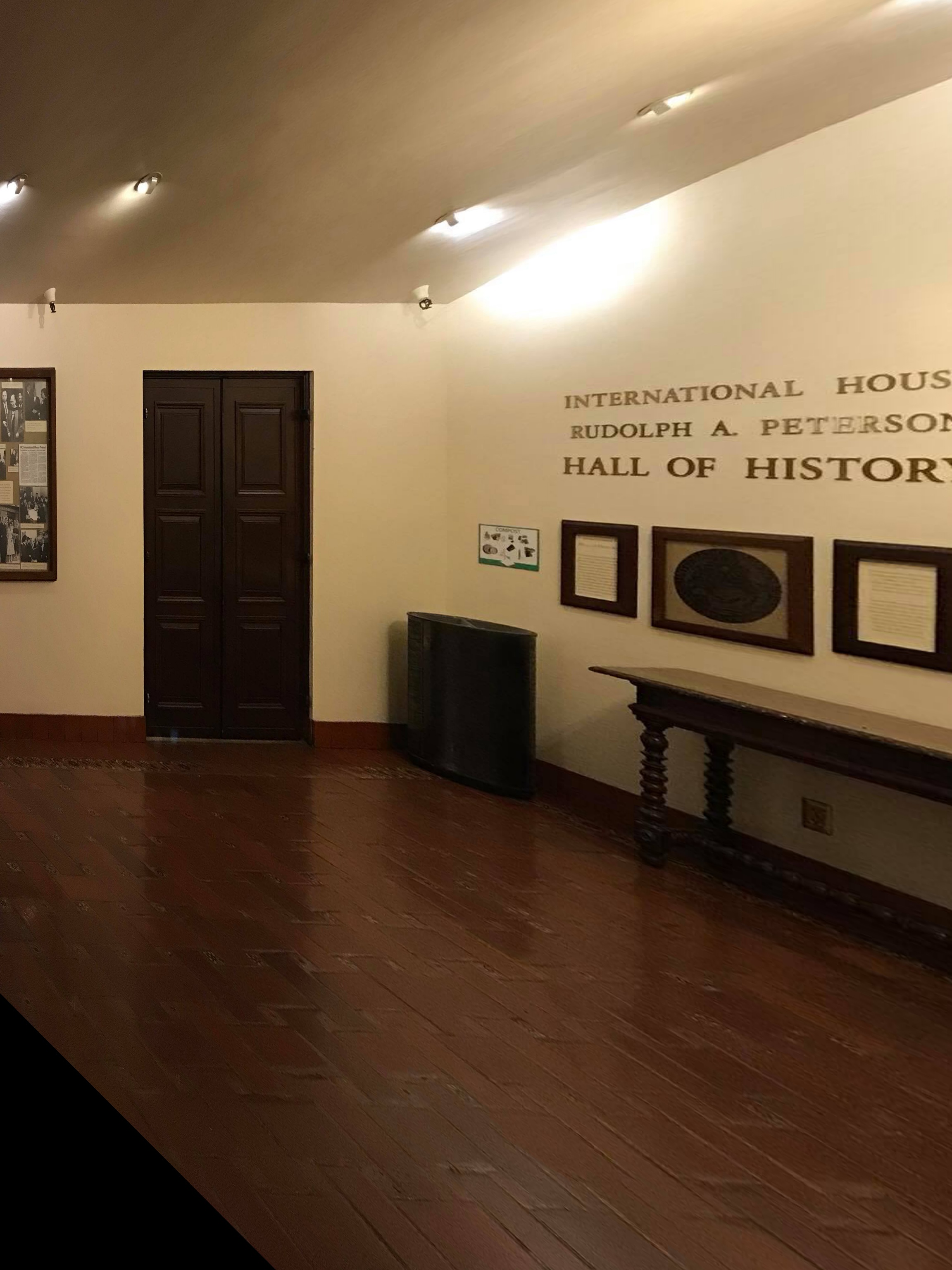
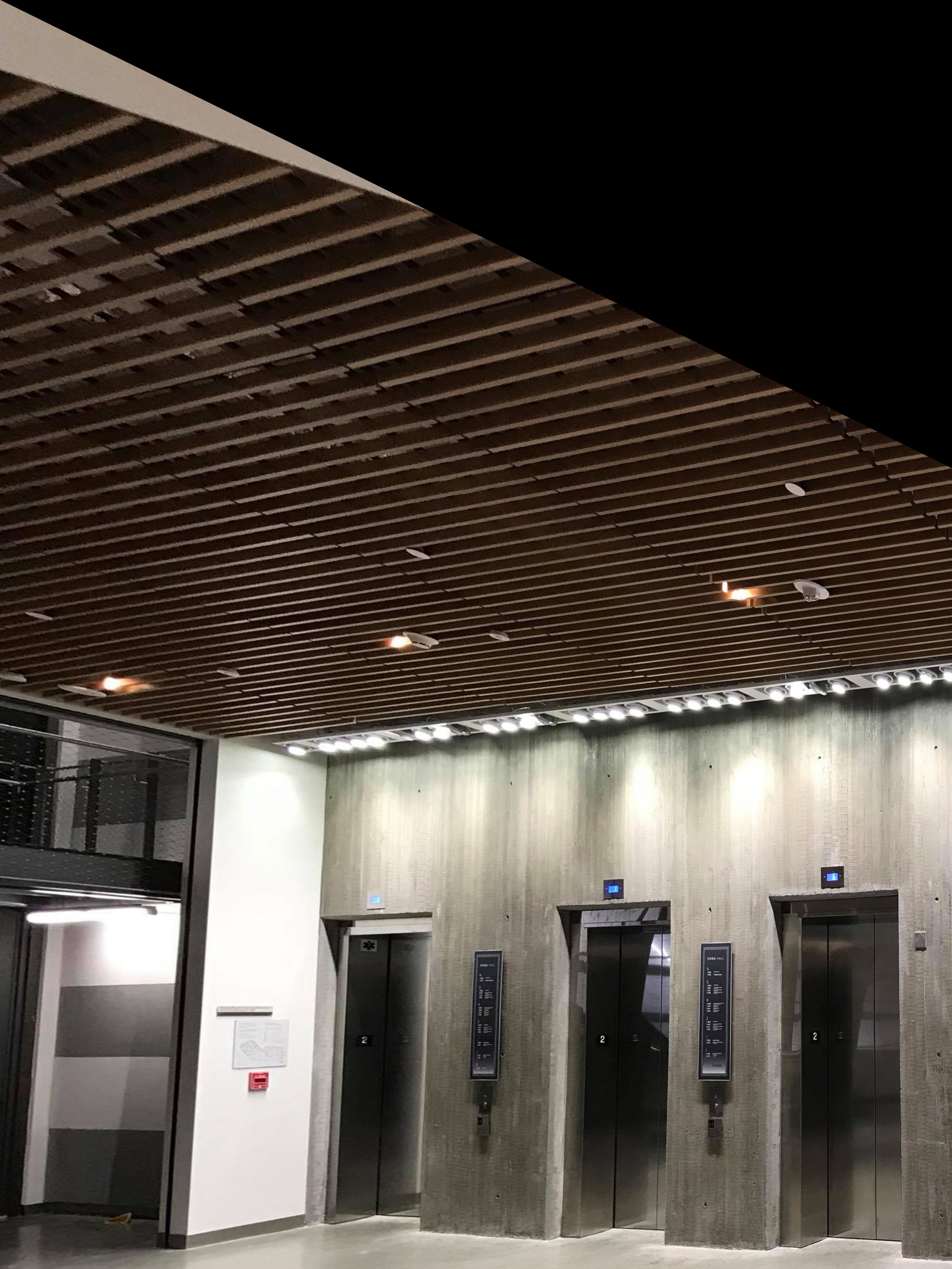
For the first part, we shot and digitalized pictures. To do this, I just used my iPhone 7 plus camera which has pretty good resolution.
Here are the images that I gathered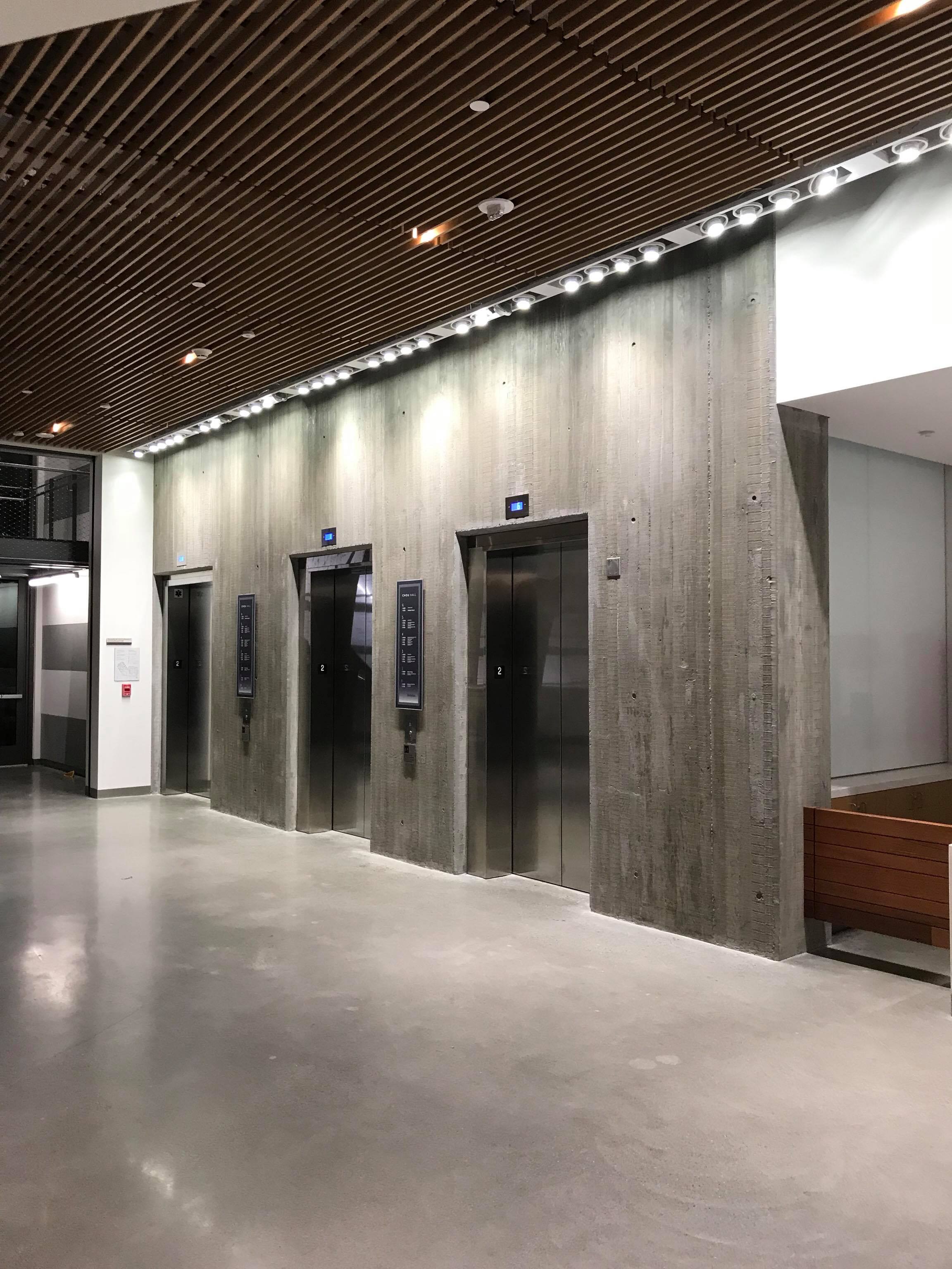
Part2: Homographies
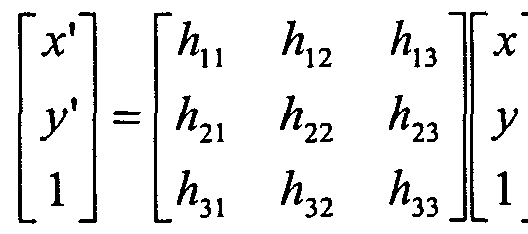
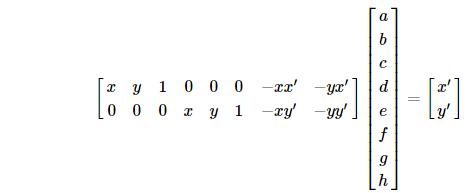
For this part, I calculated the homography matrix using the 2 equations Hp = p' and Ah = b, where H is the transformation matrix, p , p' are corresponding points in two images, h is a vector of 8 degrees of freedom, and A is the matrix such that x' = ax + by + c - gxx' -hyx' and y' = dx + ey + f - gxy' - hyy'. The Hp = p' equation took on the form below. Ah= b takes on the form of the other equation.
Part3: Image Warping
Using our homography, that we calculate in the previous part, we were able to manually pick corresponding points and use skimage inverse warping to produce a warped image.
Part 4: Image Rectify
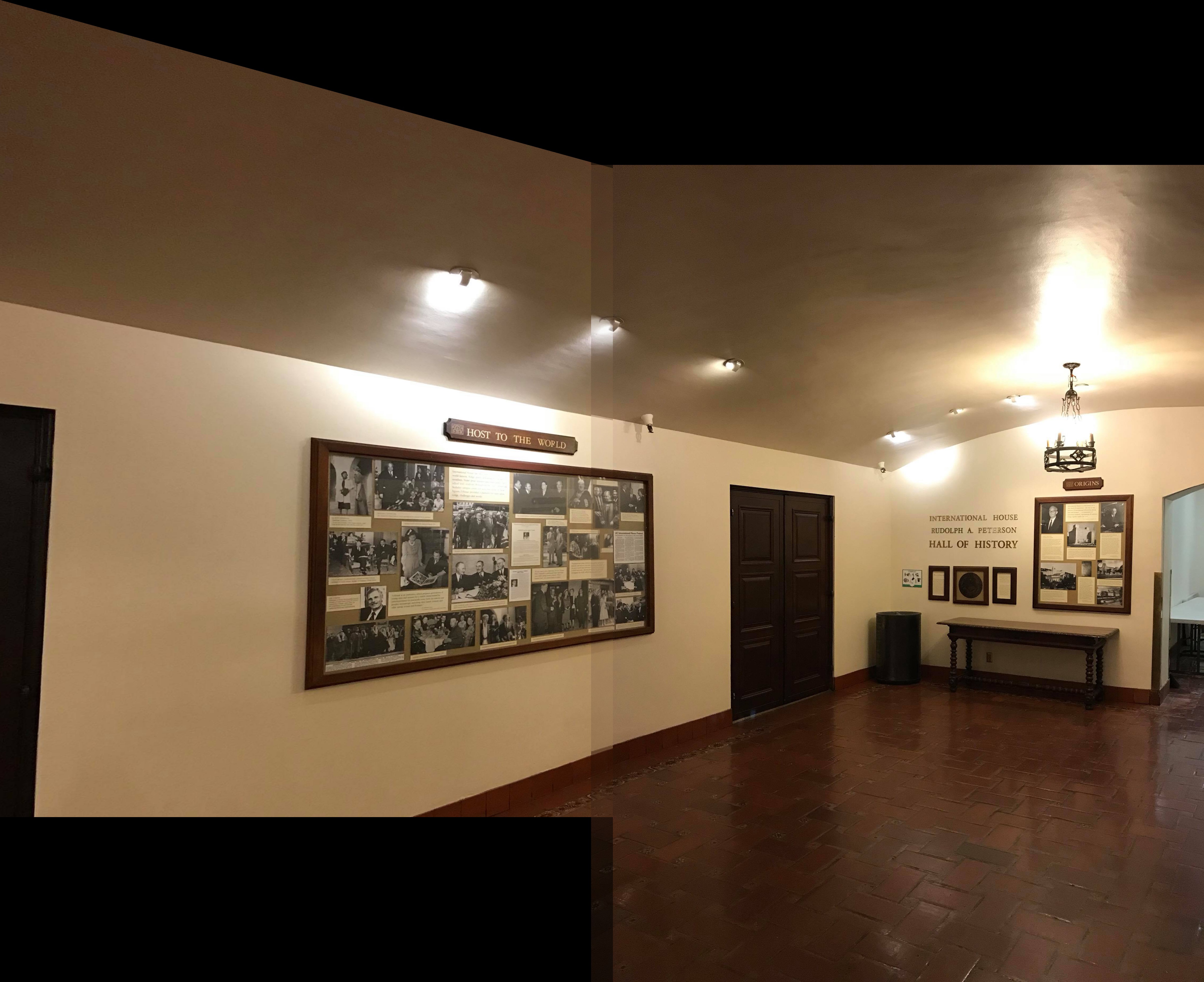
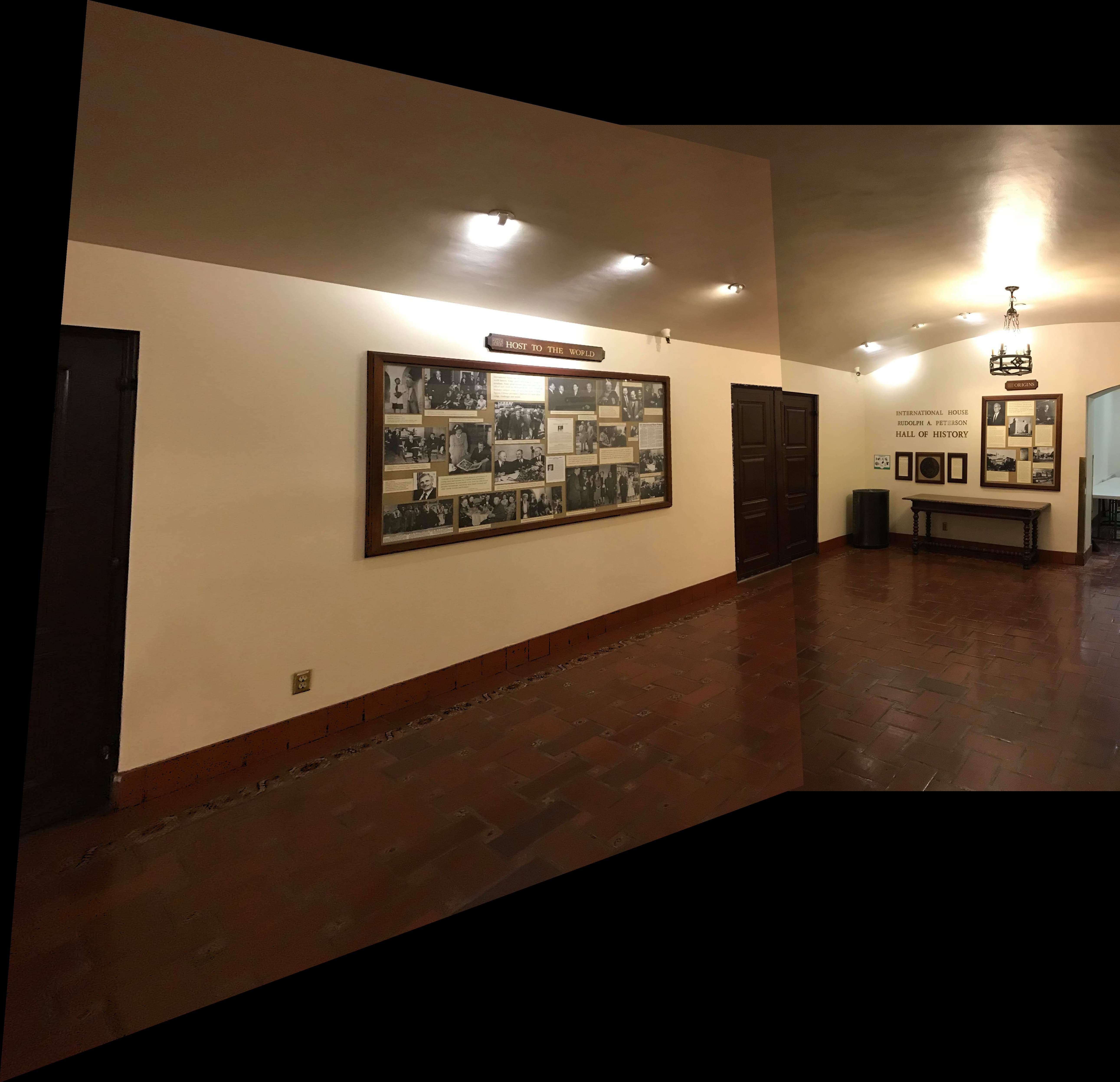
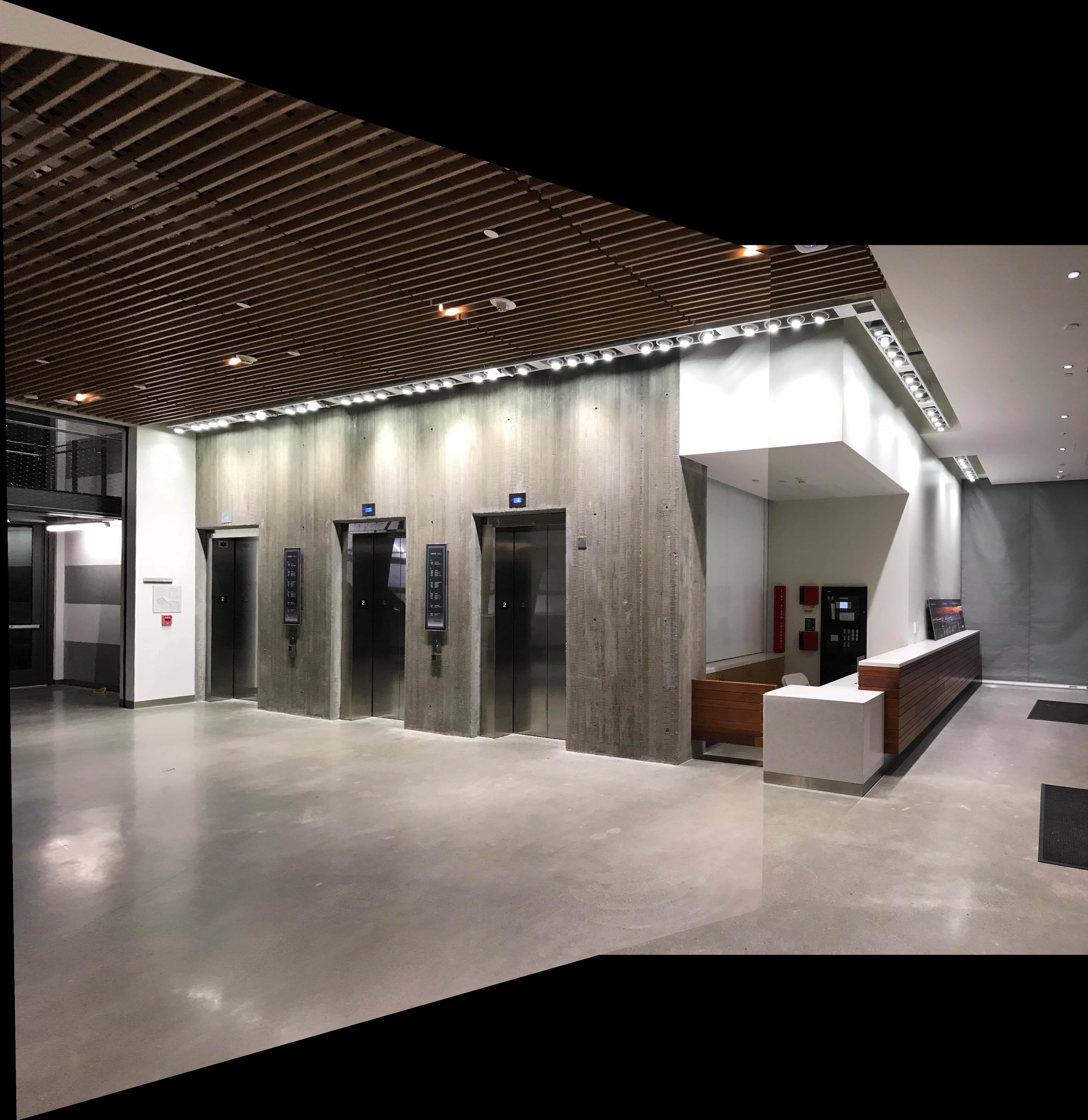
Using our image warping tool, we can change the image perspective by selecting points in the image and warping them to their physical shapes. An example below is that we change the perspective so that the door is rectified. In the other example, we change the perspective such that the elevator doors ar rectified
Part 5: Mosaic
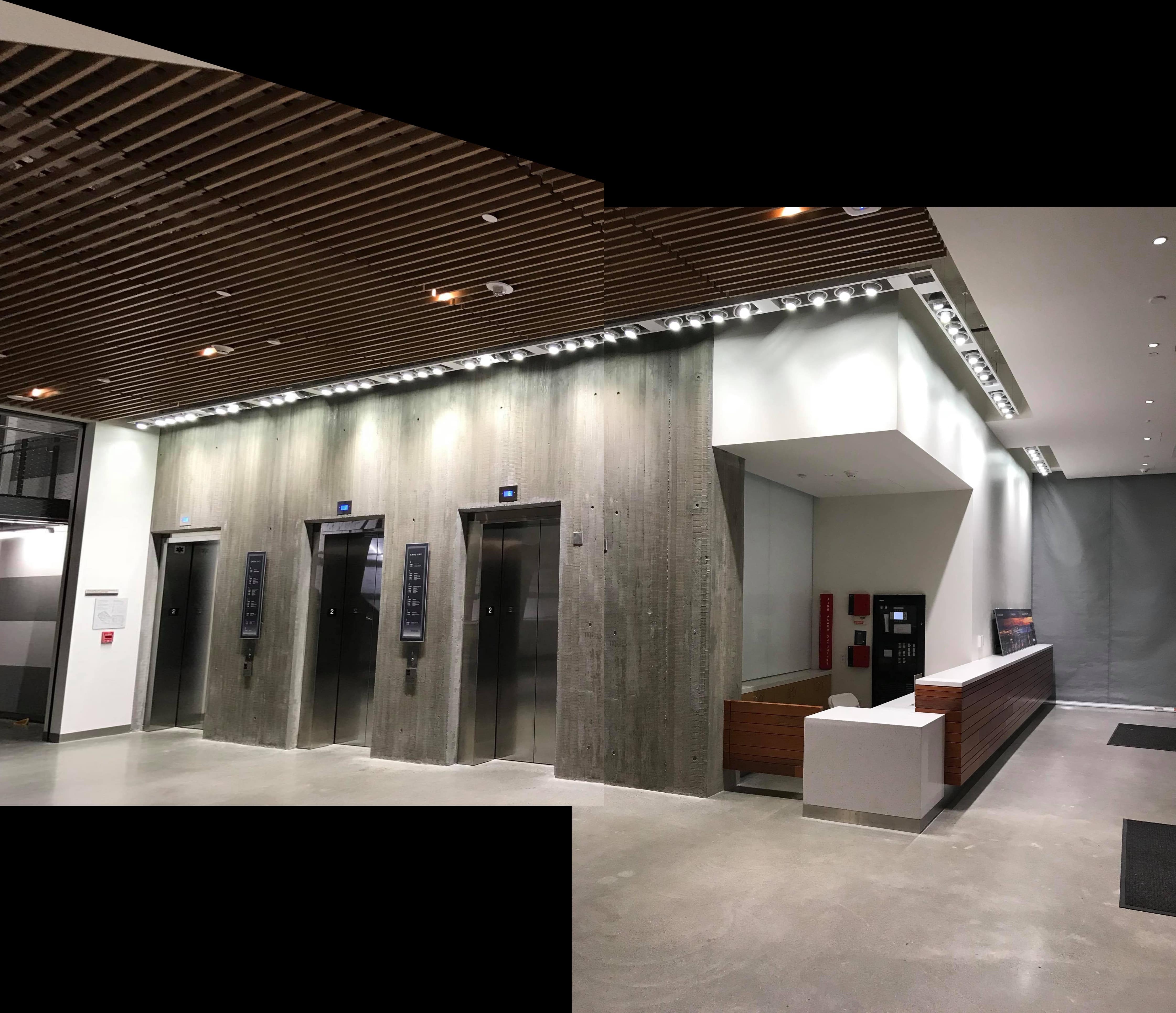
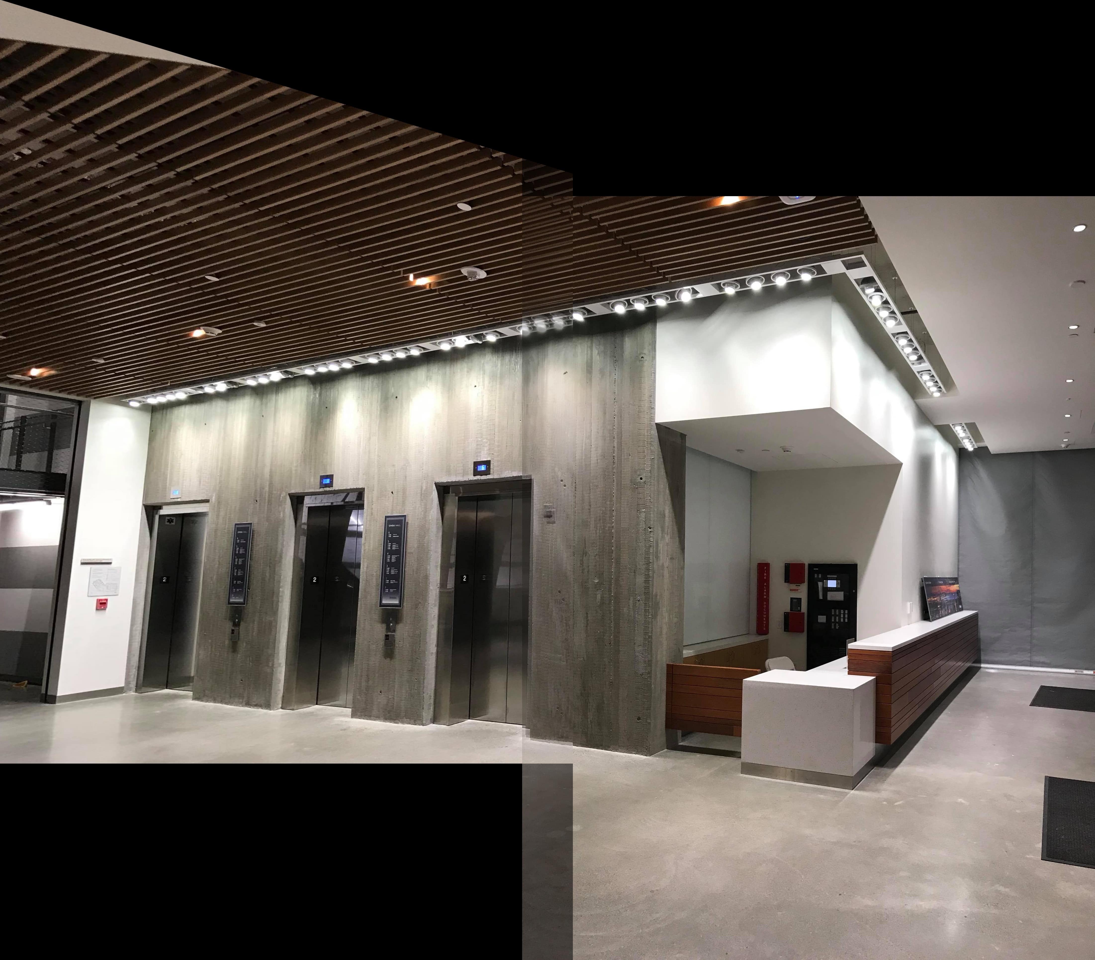
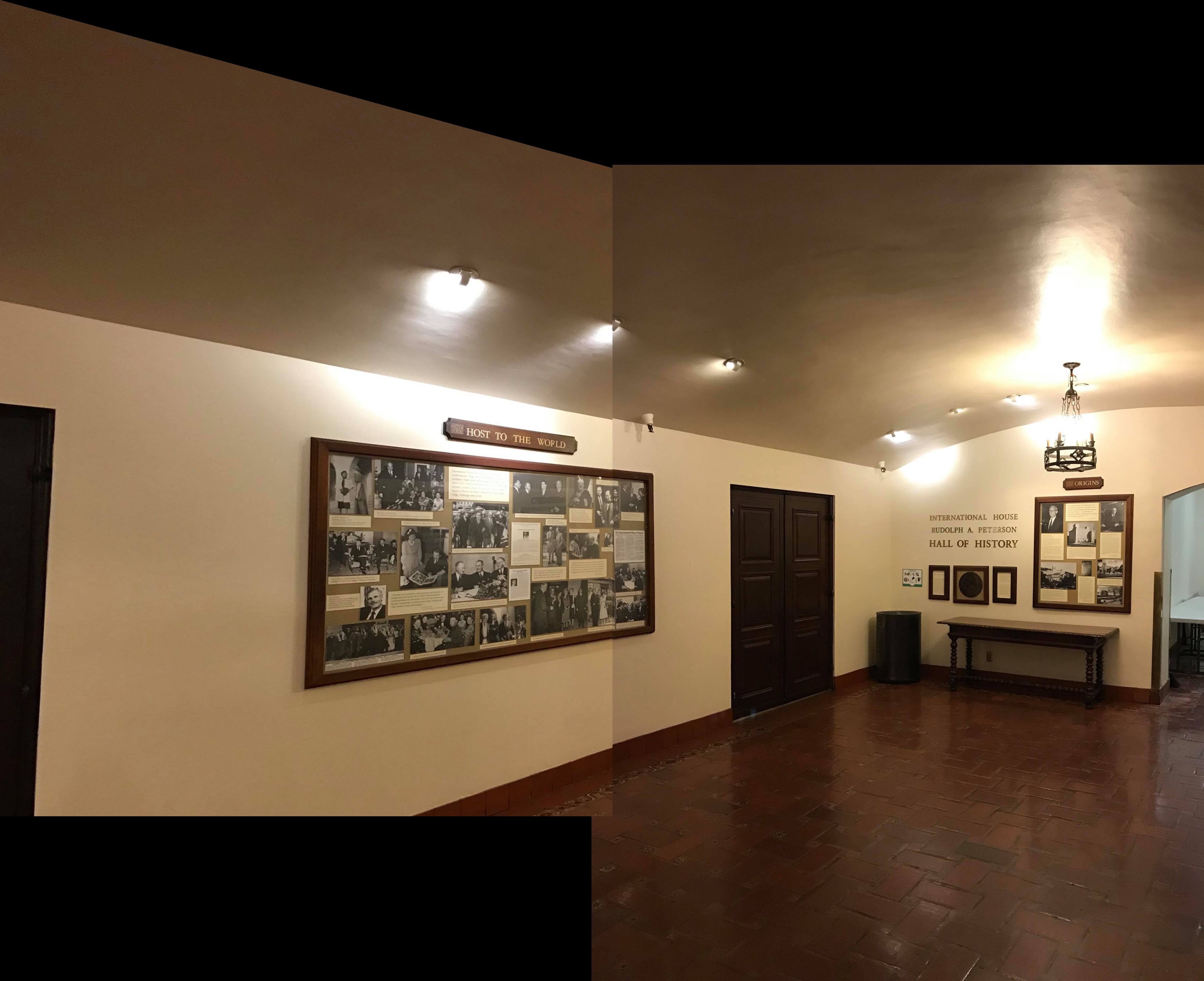
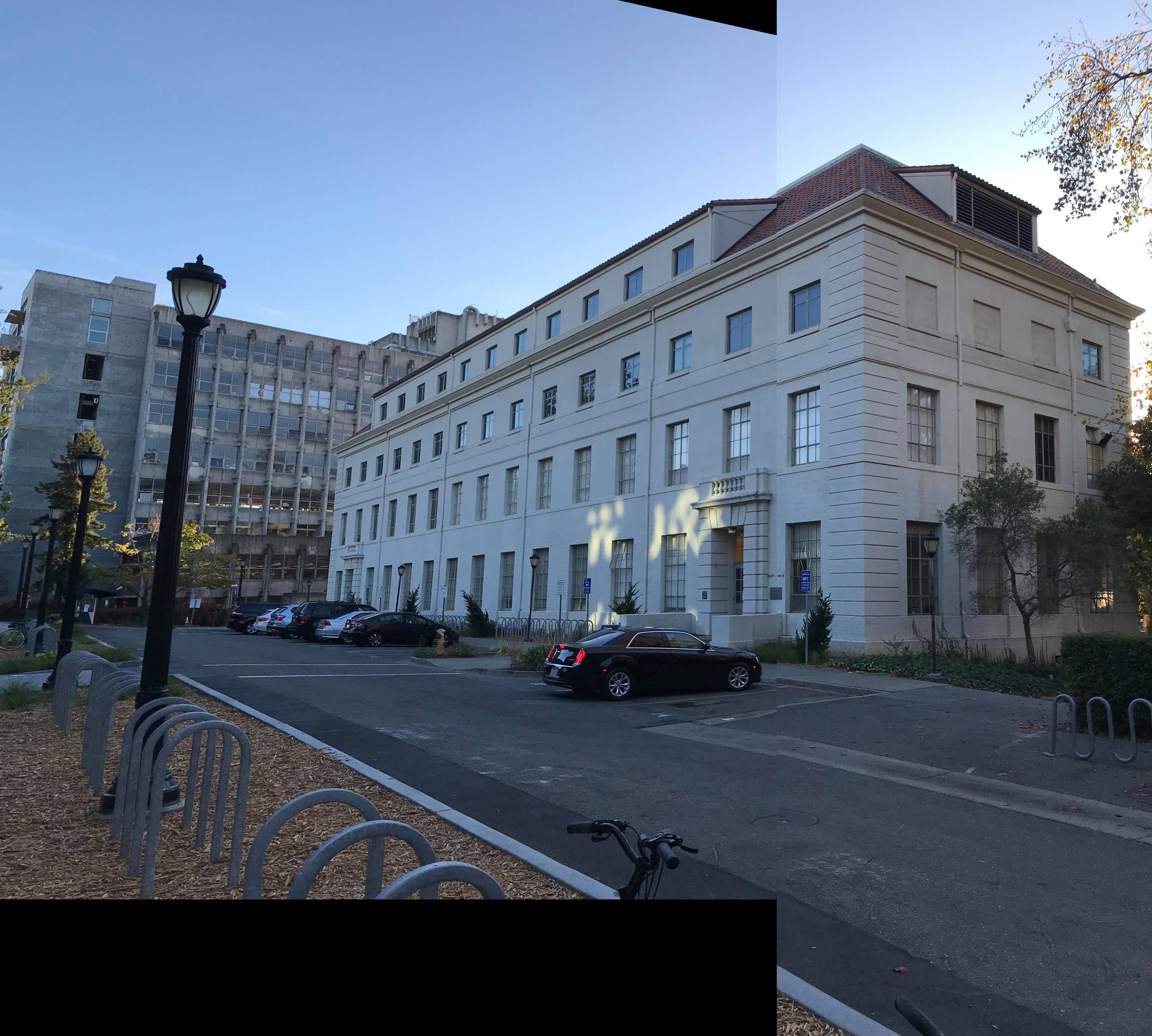
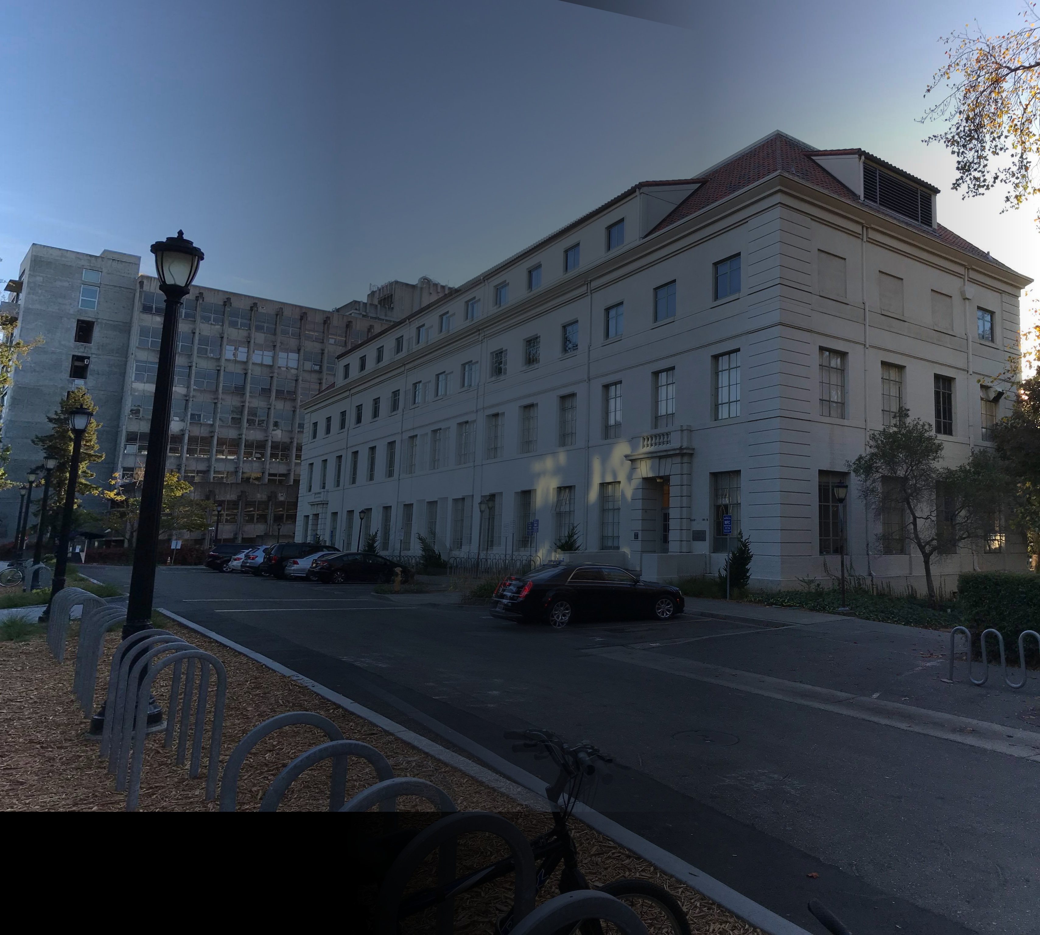
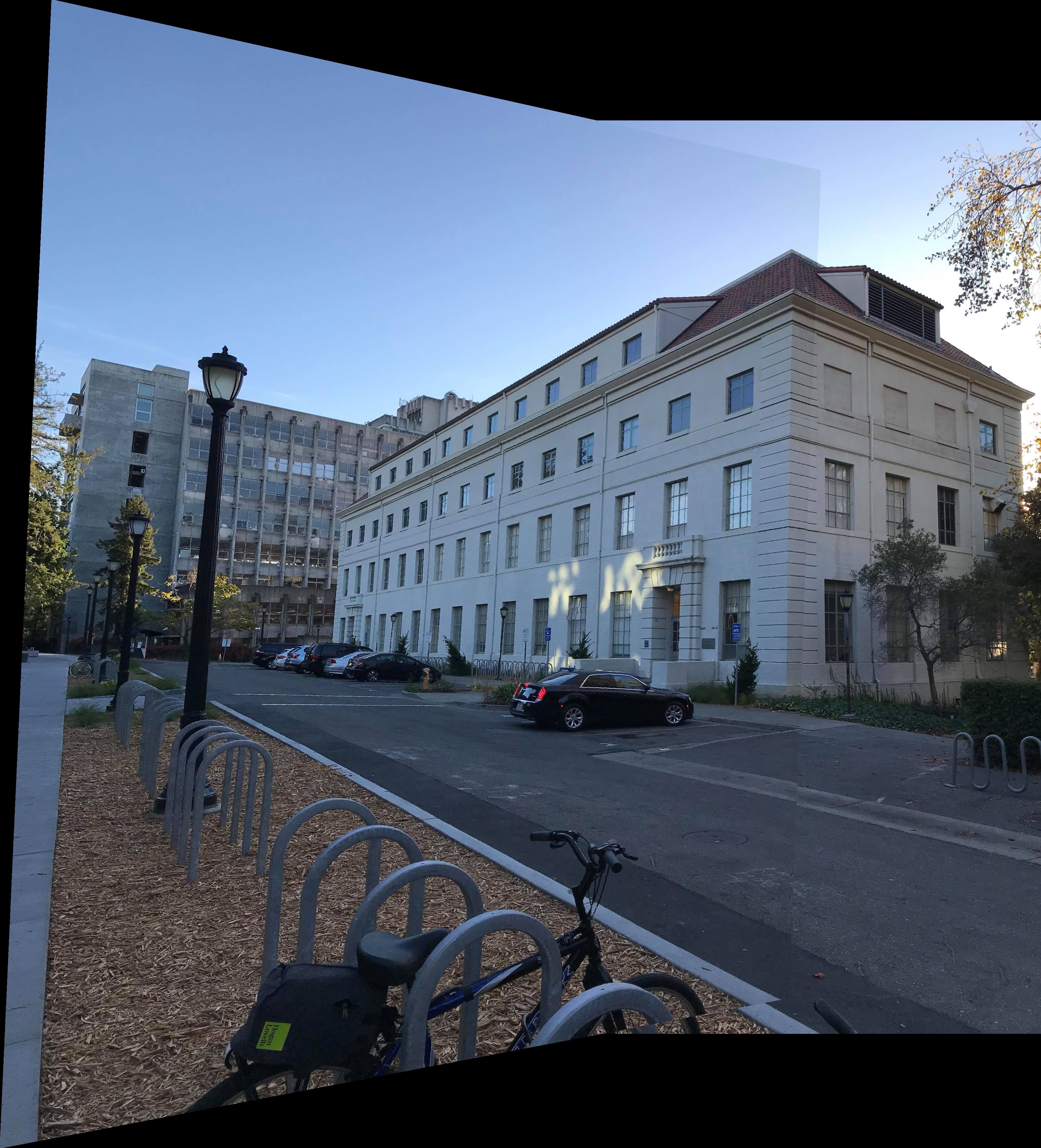
Finally, with our images warped to the perspective of another image, we were able to stitch together images to create what is essentially a panorama. Below, we can see the results of using average blending, and linear blending using a mask to blend the images.
Part 6: Summary
By finding the homography, this allowed us to take image points and transform them to another space. This allows for us to change the perspective of an image. By alteringn the perspective of an image, we can stitch together a set of images that were taken from the same spot but with different perspectives in order to create a larger image.
Part B: Overview
The goal of the second half of the project was to automatically find the correspondence points that we manually picked in part 1. Corners can be automatically detected in using a harris corner detector. Feature descriptors are then extracted from these points, and are matched across the images. We can then use RANSAC to compute a homography. After finding this homography, we do the same thing we do in part 1 and stitch the image to create a mosaic.Part 1
For the first part, we were able to use the harris corner detection provided by the spec in order to find correspondence points. By using Adaptive Non-Maximal Suppression, we can greatly reduce the number of points that we gather.
Part2: Description Extraction and Feature Matching
After we get our set of points from the previous part, we perform extraction on these points to get image descriptors.These image descriptors will help us match the points between the two images later on. We compute a point's descriptor by taking a 40x40 square centered on the point, blur and downsample the square to an 8x8, and then normalize it. Once we have these extractions, we can then perform feature matching. This is done by taking the SSD between every feature in the first and second image using the dist2 function provided by the spec. Finally, we take the ratio of the nearest neighbor to the second nearest neighbor and use a threshold of 0.4 to filter out invalid matches.
Part3: Ransac
Now that we have a set of feature matches, we can use the RANSAC algoirthm to compute the homography in a robust manner. We sample four matches at random and compute a homography from this result. Then, we use this homography on all the features and calculate the difference between this and the true values. Afterwards, we keep track of the inliers that lie within the threshold that uses the euclidean distance between points. We run this process x amount of times (I used 5000) and take the homography that results with the highest amount of inliers. With the best homography, we then do what we did in Part A of the project and just warp and stitch the image.
Part 4: Images
I did not see a huge difference in my autostitched results and my manually stitched results. Two things could have possibly occured. Either I did not take the best pictures for autostitching, or my algorithm wasn't perfect. The fact that I was able to achieve better results with manual stitching makes me think that I could have drastically improved my autostitch.
Part 5: What I learned
I learned that autostitching is a lot more powerful then manual stitching because autostitching is done using linear algebra with significantly more operations. I also learned about the concepts of RANSAC and harris corners. Finally, i got to see what features of an image are distinguishable based on where their harris corners are located.