CS194 Project 6: Image Warping and Mosaicing
Matthew Waliman, cs194-26-afq
In this assignment we warp images into mosaics to generate panoramas. There are two main parts: 1. Image Rectification, the core utility to image stitching, and 2. Blending to create mosaics.
I. Image Rectification
In order to align the images we have take into account that the camera looks at the same scene from different perspectives, in essence taking a project transform of the scene. A Homography is a projective mapping between two planes with the same center of projection, the camera axis. A projective transform allows mapping between any pairs of quadrilaterals. It does not preserve parallel lines but does straight lines. The projective matrix His below.
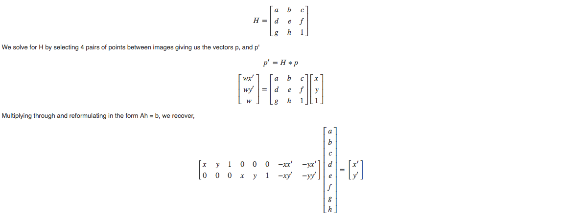
We have 8 unknowns. Now it becomes clear why we needed 4 pairs of points in order to solve for h or H. We then plug A and b into a leasr squares solver to recover an H that best fits the specified points.
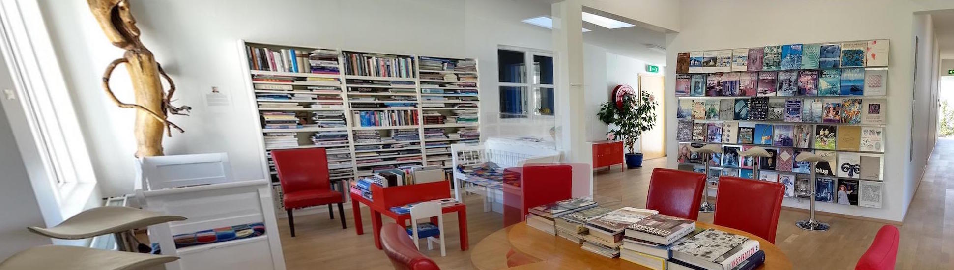
Here are the images I will be using to demonstrate rectification.
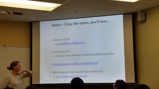
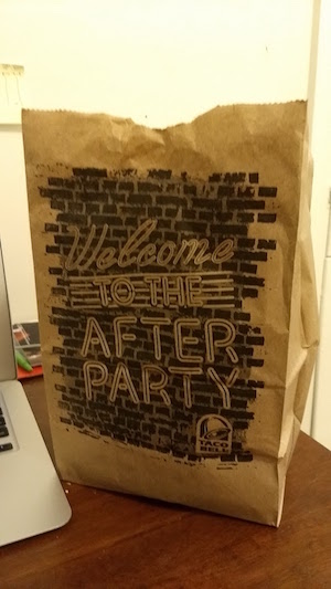
First I chose the 4 corners of objects I knew the geometry for. Here, I chose the slide and a face of the paper bag. Then I just 4 arbitrary correspnding target points at right angles in the rectified canvas space. Then I image warped using the bilinear interpolation we used back in project 4. These are the results. One thing to note is that the transform will match the four points to the four specified target points, however the rest of the image will be projectively transformed in different directions, almost always verging into the negative axes. In order to account for this in the future, we apply shifts into the positive quadrant so that we are able to view more of the image.
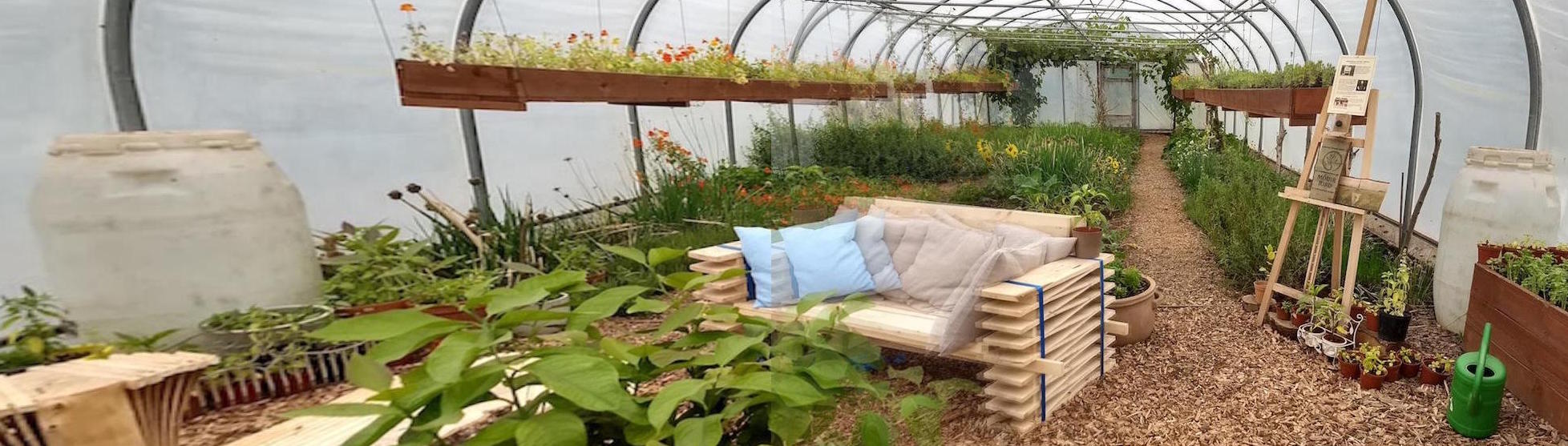
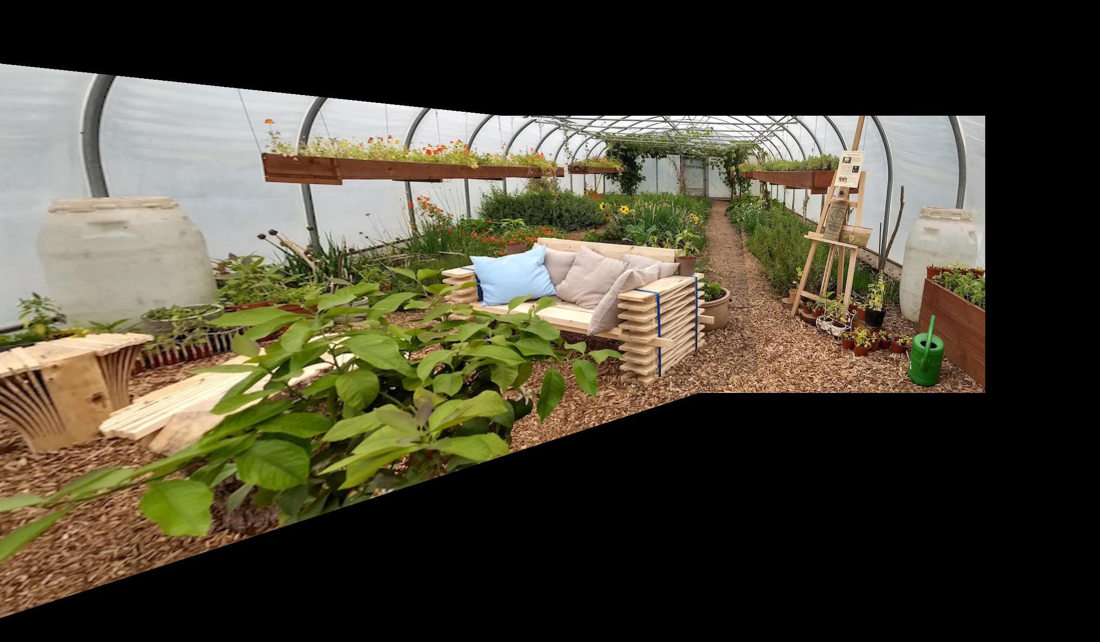
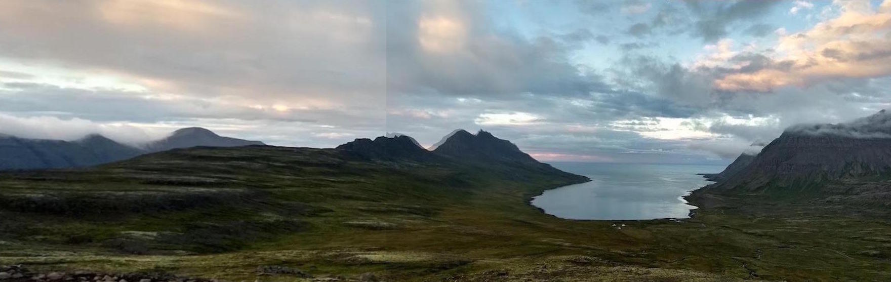
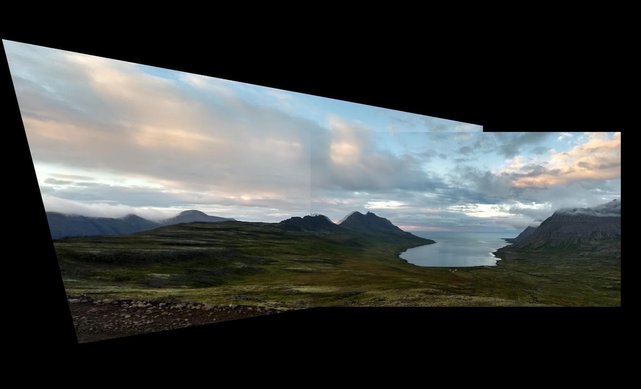
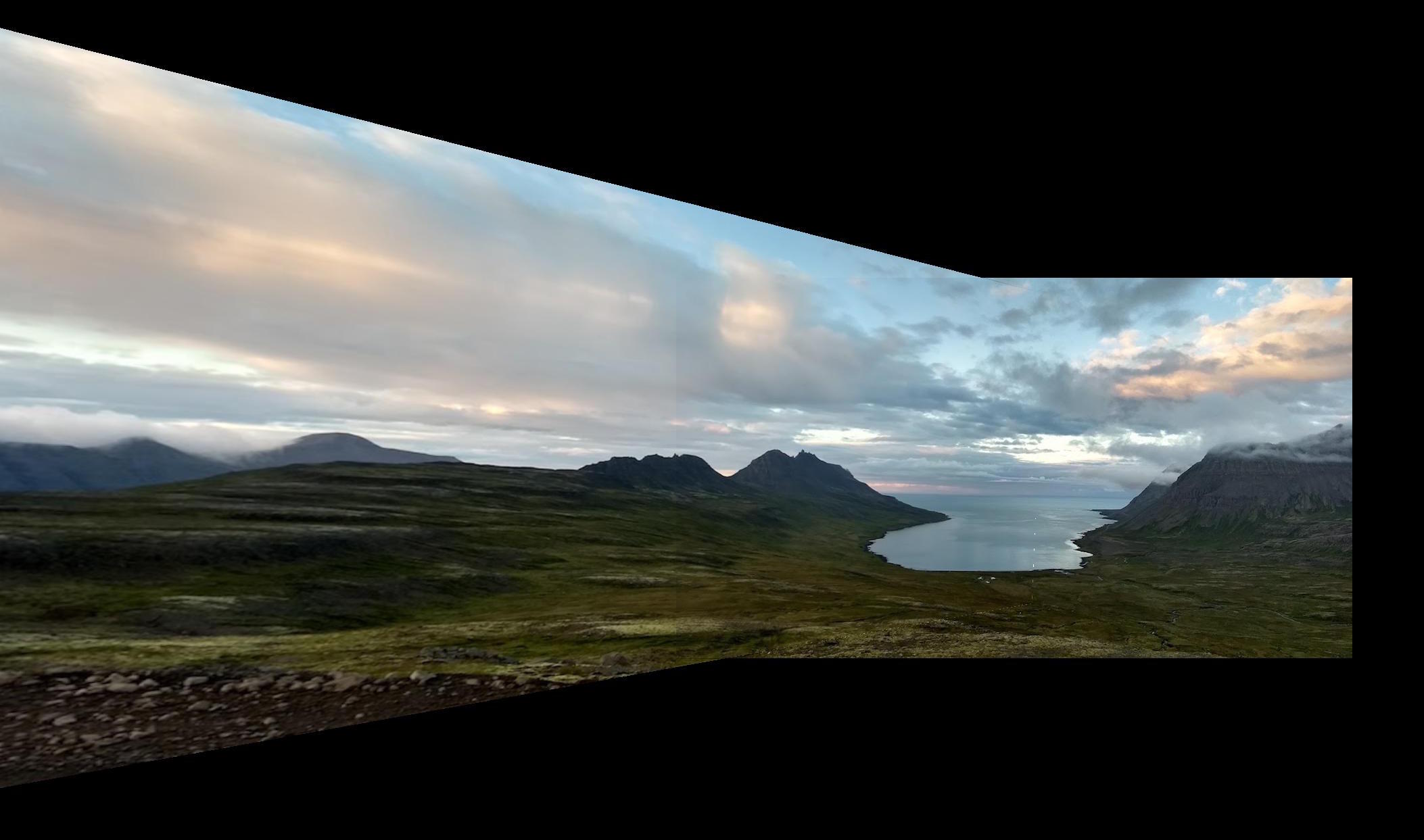
II. Creating Panoramas
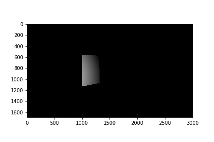
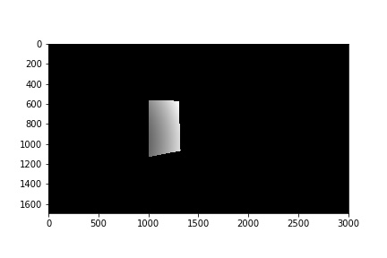
There were a few challenges to applying multiple projective transforms and combining them. The first was where the each transformed image should go in the final image. In all panoramas shown I warped one image into the plane of the other. Then I chose a canvas approximately 3 times the size of the base image and applied the transforms. Finally, blending the two images proved more difficult than I originally imagined. I ended up using linear blending. I calculated the overlapping areas of each image and calculated the distance from each respective image center. This became a scaled alpha, with which to blend each image. The respective "masks" for the overlapping region are shown.


III: Autostitching
In order to implement autostitching, we need to find a way to match up the images automatically. We approach this by automatically detecting and matching features to create pair correspondences between the images.
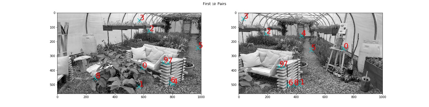
Harris Interest Points & Adaptive Non Maximal Suppression

First, we need to generate features of interest. Here, we used the Harris corner response to generate interest points (marked in red) at corners and edges. You'll notice that we only collect Harris points 20 pixels in from the border, this is so that we can easily collect 4x40 feature patches later on. There are a lot of Harris pts, so we need some way to reduce the quantity of pts while retaining only the ones with the highest Harris response. In order to do this we perform Adaptive Non-Maximal Suppression, which works by choosing points (in cyan) that are furthest away from their closest neighbors with a sufficiently high Harris value. Let's break that down a bit.
- Find the SSD between all Harris points, we'll denote these as points as h_i, and all other Harris points in the image as neigbors, h_j.
-
For each h_i, get rid of all h_j whose Harris value H(j) falls below a fraction of H(i),
c_robust= 0.9. - Out of these h_j with sufficiently large Harris value, find the closest one. We'll designate that the nearest neighbor.
- We now have a nearest neighbor with good Harris value for each point h_i. Find the SSD between each point h_i and its nearest neighbor. We want the top 500 pts that are furthest away from their nearest neigbor, giving us evenly spaced interest points.
Multiscale Orientation Patches
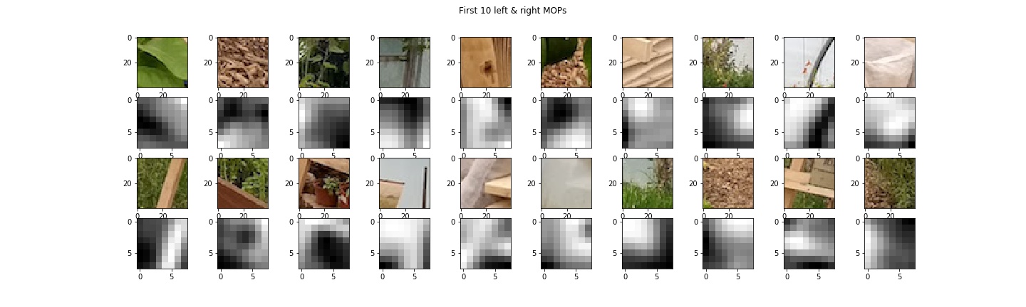
Now that we've narrowed down our points a bit, we need to be able to compare these features to each other in order to perform matching. This part is quite simple. We generate 40x40 patches around each feature, blur with a gaussian to reduce noise, bias/gain normalize and finally subsample by a factor of 5 to produce 8x8 feature descriptors. I actually didn't implement the Orientation part of the MOPs, but the matching works well enough.
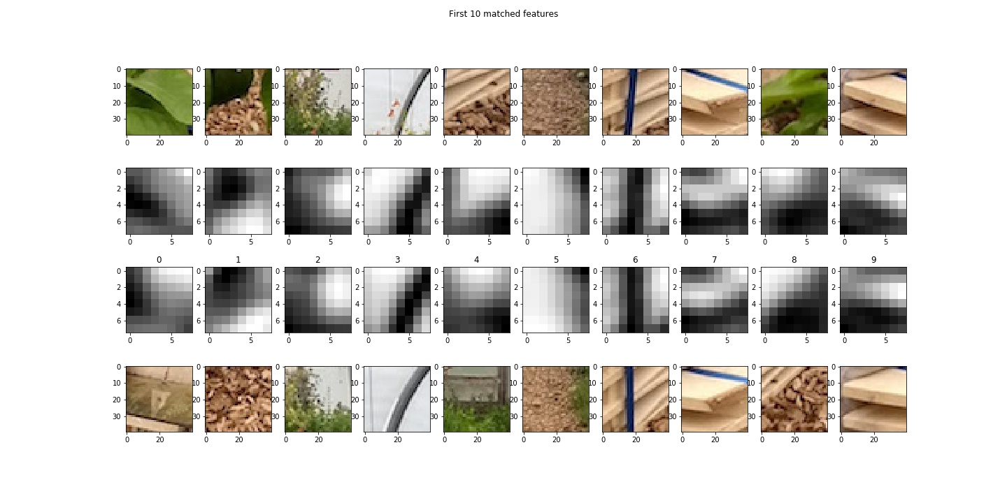
Feature Matching
To match these feaures/patches against each other, I followed the following steps.
- Find the SSD between all patches in the left image and all patches in the right image.
- For each feature, find the two patches that most closely match(smallest SSD).
- Calculate the distance between each feature point and its 2 nearest neigbors. If dist(nn_1-i) * frac > dist(nn2-i), exclude this feature. The idea is that there should only be one neighbor that is much closer to the feature point than the rest, so dist(nn_1-i) should be way smaller than dist(nn_2-i). I used
frac= 0.67 - Collect the remaining features and their nearest neighbors
Below are a few of the pairs found. As you can see, a good number of them are correct, but we still need to remove the false matches.
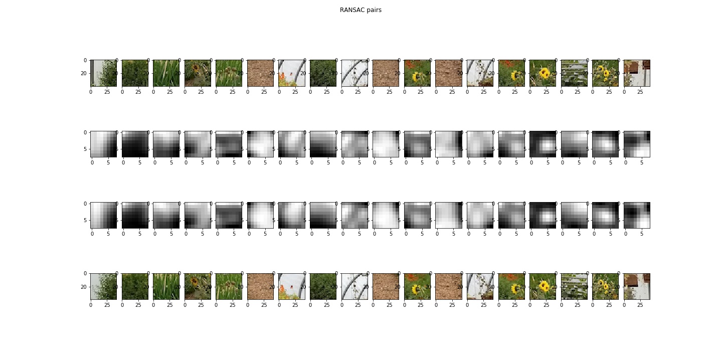
RANSAC
To perform the final winnowing of the points, we use RANSAC.
- Randomly pick 4 pairs of fearure points.
- Compute the exact homography of these points, H.
- Apply H to all points in the the left image.
- Find the distance,
| p'_i - H*p_i | - Compute inliers, or points where the distance is less than some pixel value, I used 10. Choose the set of features that had the greates number of inliers, and recompute H with all feature points.
For 10000 iterations
This algorithm is very robust, reducing the matches to the ones you see below.
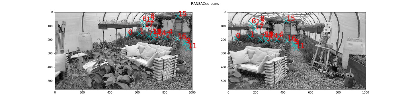
Now that we once again have pairs of correspondences, we are ready to mosaic images!
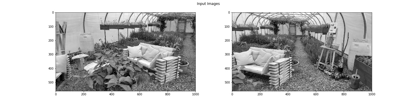
IV: Manual vs Automatic Mosaicing
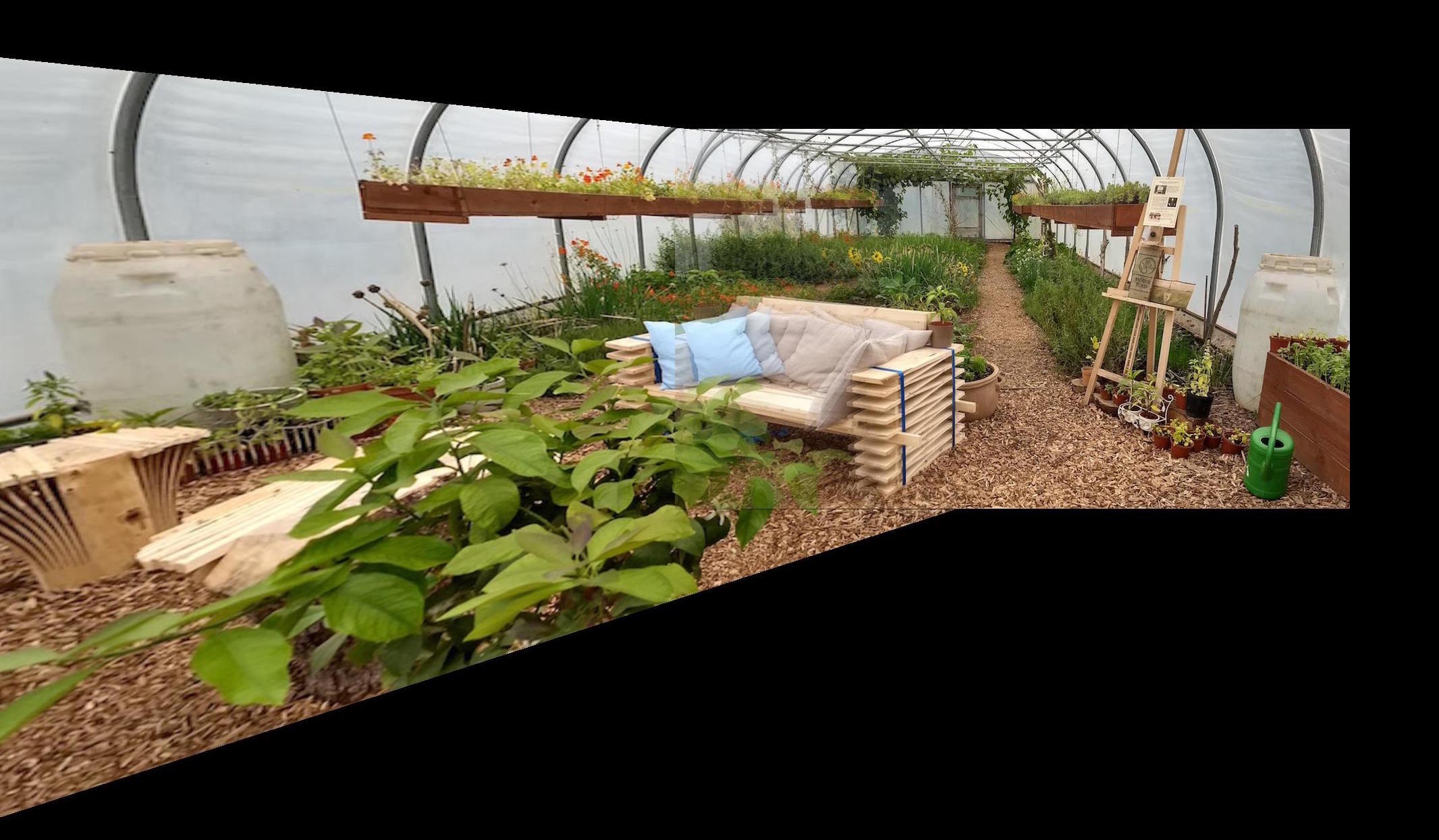
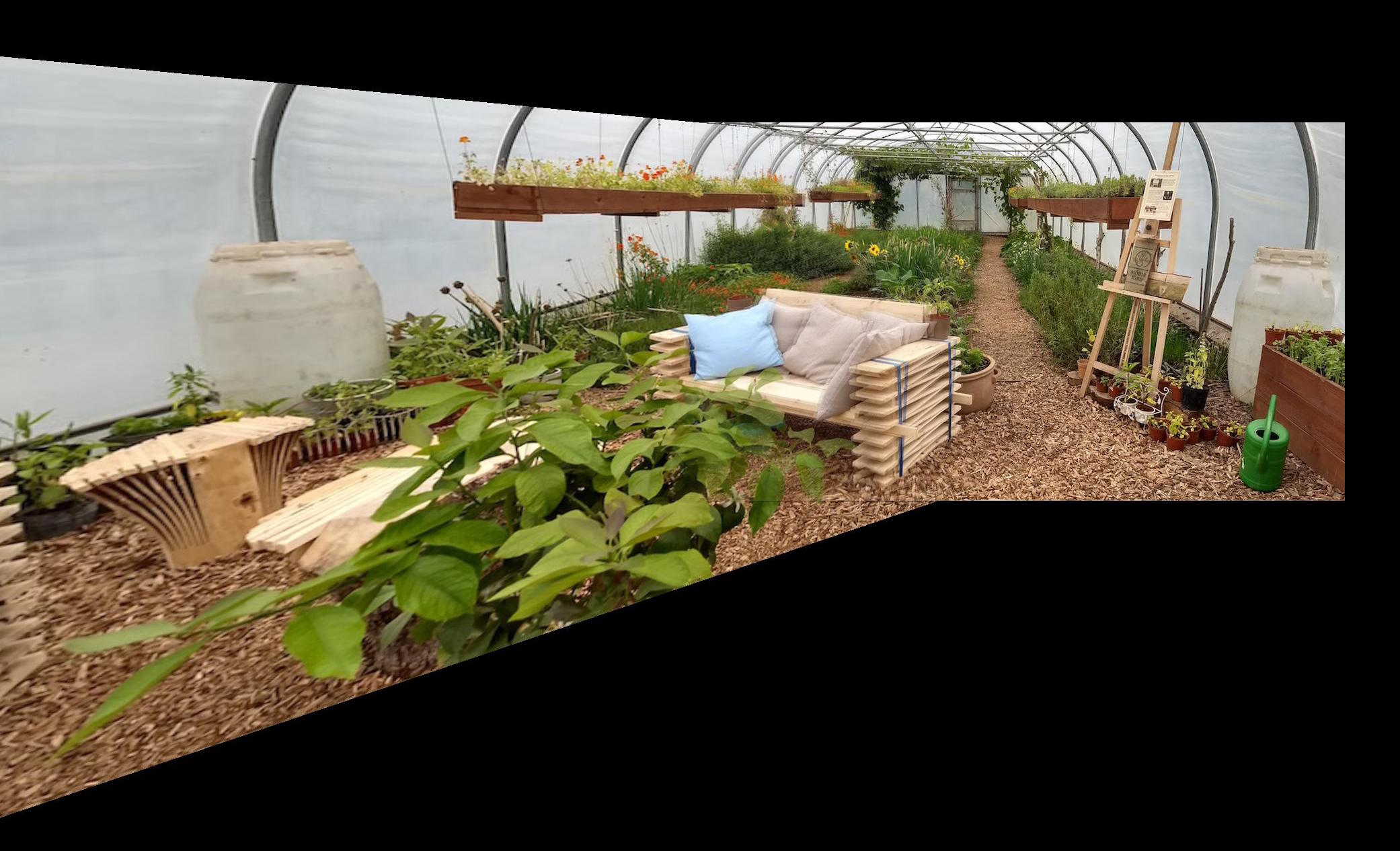
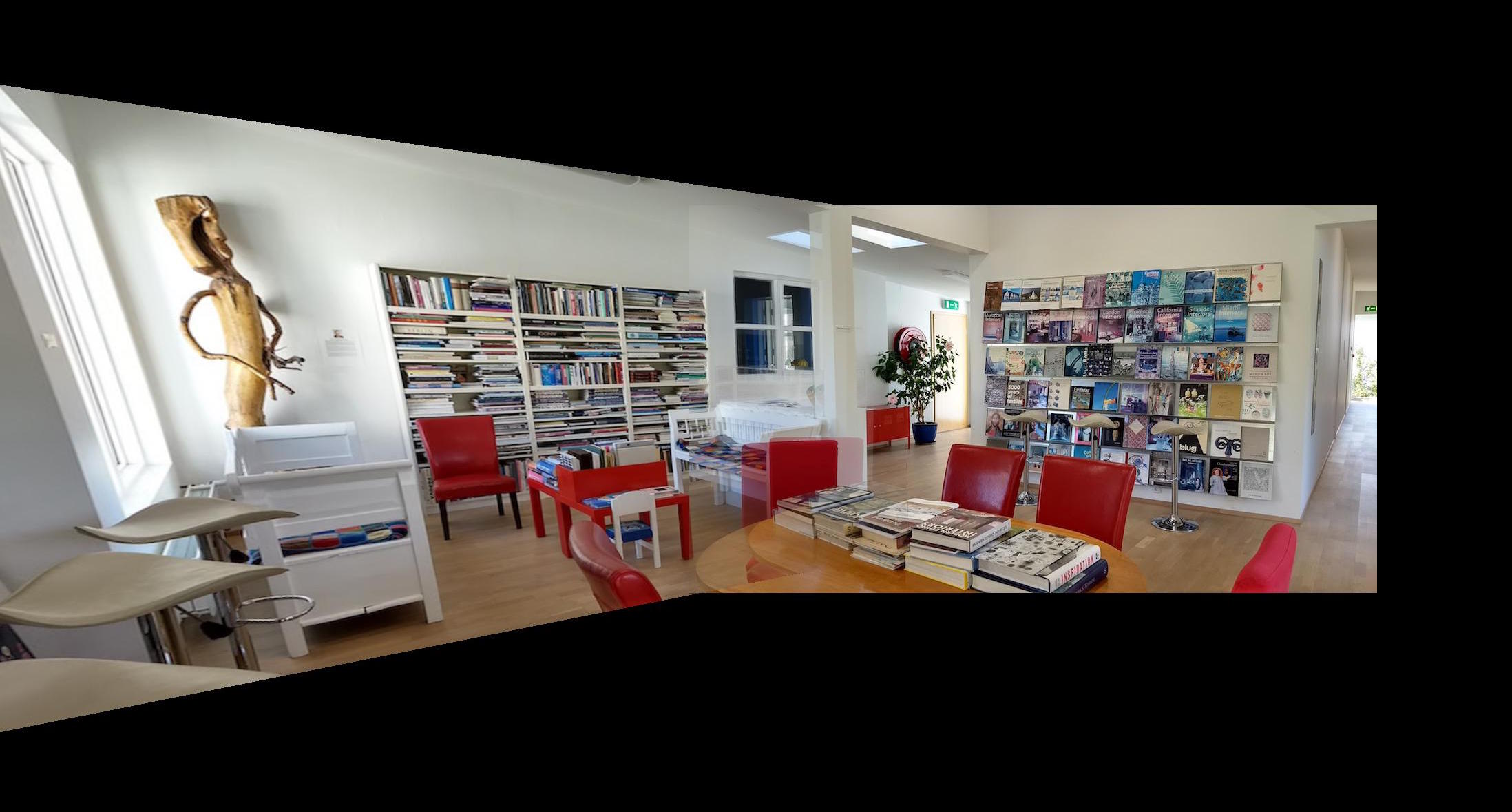
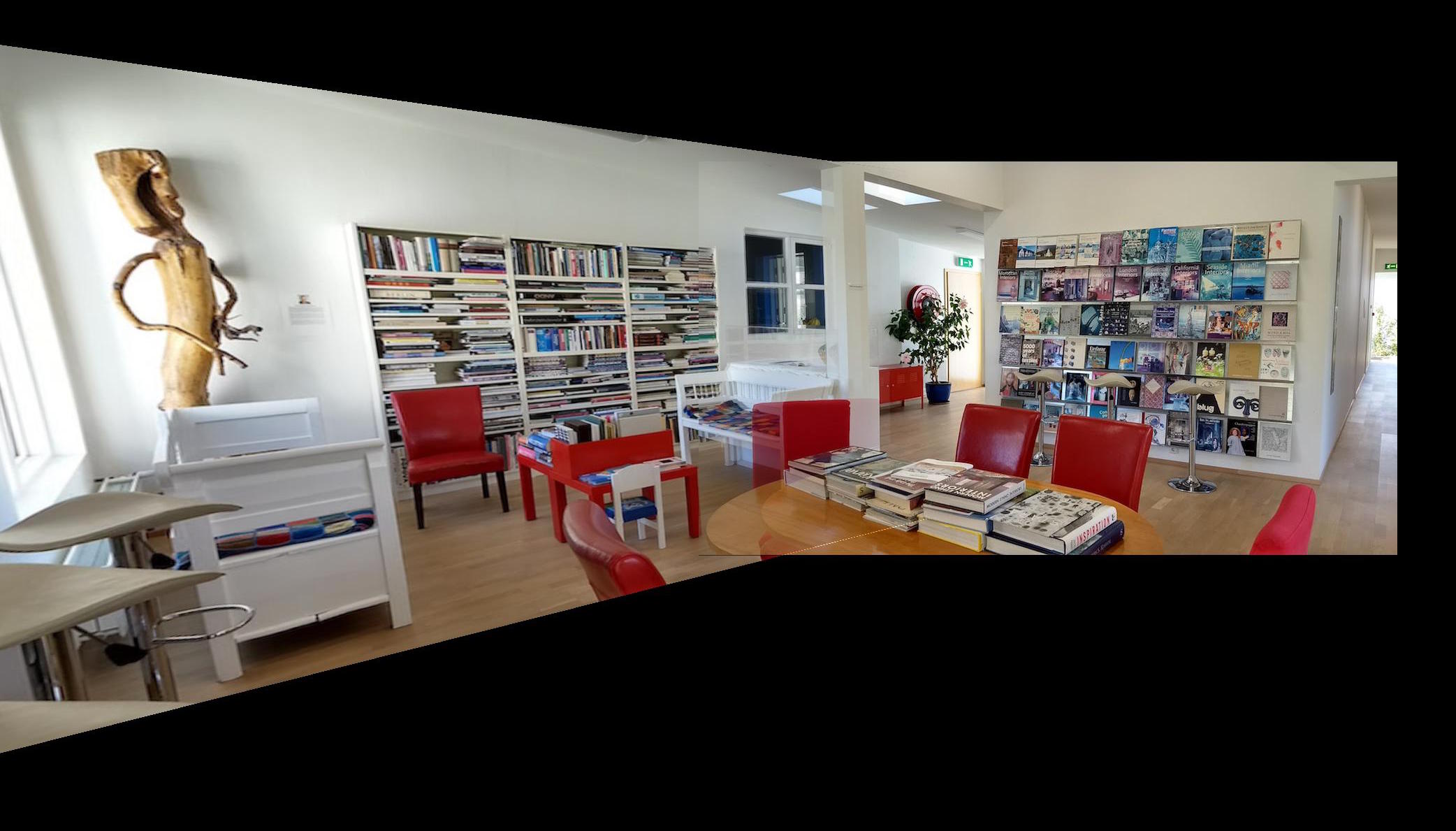
Impressively, the autostitching outperformed manual selection of feature points every time.
V: Conclusion
I really enjoyed learning how to autostitch pictures together.
