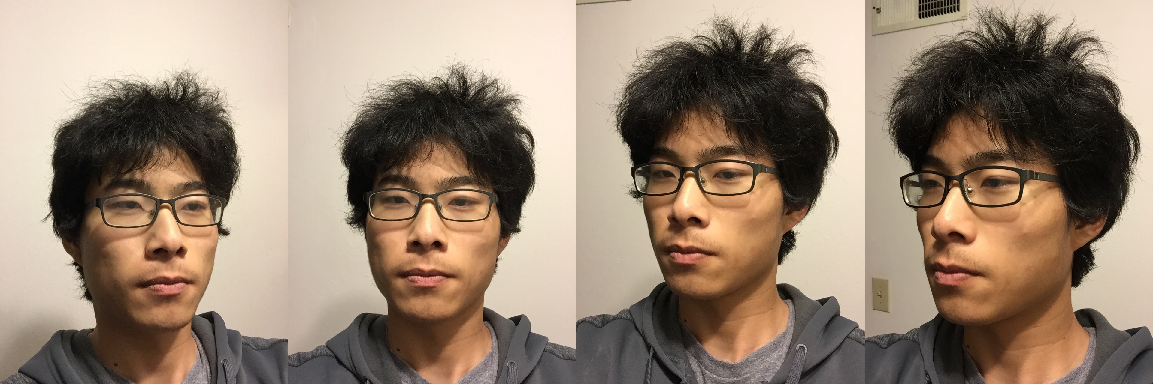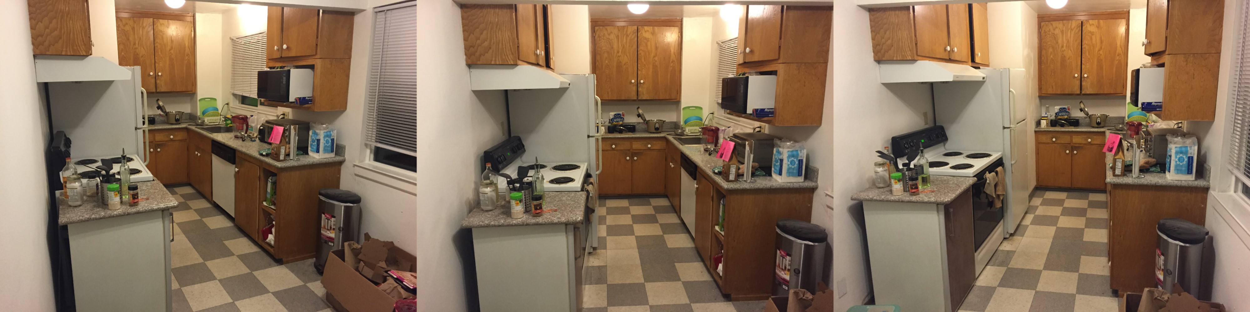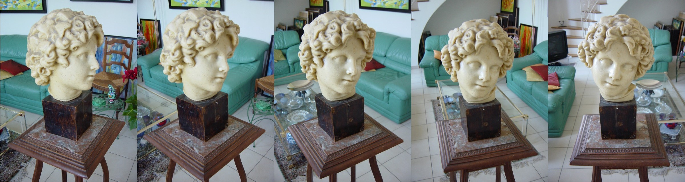
My code takes in several 2D photographs of an object from various angles as input, and it outputs a dense colored 3D point cloud that captures the structure of the original object.
This project mostly follows the steps outlined in "Multi-view 3D Reconstruction for Dummies" by Jianxiong Xiao.
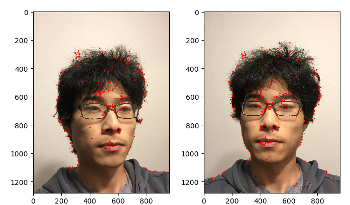
Somewhat similarly to the homography matrix, the fundamental matrix relates the corresponding points in a pair of images. Let \(x_1\) and \(x_2\) be corresponding points in two images. Then the fundamental matrix \(F\) is a 3x3 matrix such that \(x_2^TFx_1 = 0\).
For some intuition on why this relation exists, the set of all points in world space that could project to \(x_1\) forms a line. Projecting this line onto the second image plane forms another line. Thus, any point in the second image that corresponds to \(x_1\) in the first image must lie on this line, which is the set of points normal to \(Fx_1\). It can be shown that this matrix is identical for all pairs of corresponding points, and so for corresponding points \(x_1\) and \(x_2\), \(x_2^TFx_1 = 0\).
Expanding \(x_2^TFx_1 = 0\), we get $$\begin{bmatrix} x_2x_1 & x_2y_1 & x_2 & y_2x_1 & y_2y_1 & y_2 & x_1 & y_1 & 1 \end{bmatrix} \begin{bmatrix} f_{11} \\ f_{12} \\ f_{13} \\ f_{21} \\ f_{22} \\ f_{23} \\ f_{31} \\ f_{32} \\ f_{33} \\ \end{bmatrix} = 0$$ With many pairs of corresponding points, we can set up a system of linear equations \(Af = 0\) and then solve for \(F\) using least-squares.
Alternatively, we can use the 8 point algorithm. It turns out that \(F\) has 7 degrees of freedom, but it's easier just to use 8 points. We can compute the SVD of \(A\) and then take the right singular vector corresponding to \(A\)'s smallest singular value as our solution for \(F\). This solution has a norm of 1, which is pretty nice.
Actually, as is, the 8 point algorithm doesn't give very good estimations. This is because the homogeneous image coordinates in 3D space are actually very skewed. To fix this, we first zero-mean the points and scale them so that the mean norm is \(\sqrt{2}\) before running the 8 point algorithm. This is the normalized 8 point algorithm, and it gives much better results.
Finally, to estimate a good fundamental matrix from our set of corresponding points, we use RANSAC. We randomly sample 8 correspondences, feed them into the normalized 8 point algorithm, and take the estimated \(F\) with the most inliers.
Unlike in homography estimation, there is still quite a high probability of having outliers after running RANSAC. This is because the fundamental matrix, which can be considered a point-to-line mapping, is not quite as constraining as the homography matrix, which is a point-to-point mapping. As long as the corresponding point is near the line, which crosses quite a large area, it is considered an inlier.
There's another matrix \(E = K_2^TFK_1\) called the essential matrix. It's essentially the same thing as the fundamental matrix, if cameras didn't have their annoying intrinsic matrix \(K\). This means world units and pixel units are the same.
The essential matrix has some nice properties that allow us to extract the extrinsic camera matrices \([R|t]\). Its SVD is \(E = U\text{diag(1,1,0)}V^T\), and if we set the first camera matrix as \(P_1=[I|0]\), it turns out that there are four possible solutions for \(P_2\): \begin{align*} &\left[\begin{array}{@{}c|c@{}}UWV^T&u_3\end{array}\right]\\ &\left[\begin{array}{@{}c|c@{}}UWV^T&-u_3\end{array}\right]\\ &\left[\begin{array}{@{}c|c@{}}UW^TV^T&u_3\end{array}\right]\\ &\left[\begin{array}{@{}c|c@{}}UW^TV^T&-u_3\end{array}\right] \end{align*} where $$W=\begin{bmatrix}0&-1&0\\1&0&0\\0&0&1\\\end{bmatrix}$$
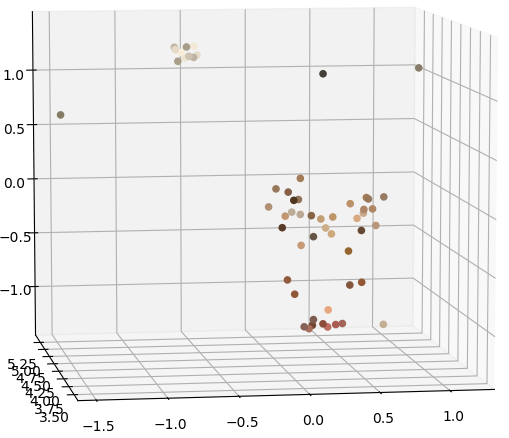
If we know the camera matrices, then given a pair of corresponding points \(x_1\) and \(x_2\), we can solve for the position of the point \(X\) in world space. (See the Triangulation section for more details.) Of the four solutions to \(P_2\), only one of them will result in \(X\) being in front of both pictures. Thus we can try all four solutions for \(P_2\), and then accept the solution with the most points in front of both cameras.
|
Now we know how to solve for relative camera positions between pairs of images, but how do we combine them together for more images? It seems that this estimation is really quite noisy, and so if we just use the camera matrices as is, the point clouds estimated from different pairs of images won't line up at all. To fix this, we have to do something called bundle adjustment.
Each estimated point \(X\) is observed in two or more images. We can reproject \(X\) onto the image plane and compare its reprojected position with its observed position. Ideally, these should be the same. Define the reprojection error to be the sum of the squared errors between the observed points and the reprojected points. Bundle adjustment is the problem of adjusting all the camera parameters as well as the estimated points \(X\) in order to minimize the reprojection error.
This is a nonlinear least squares problem, so we have to use a nonlinear least squares solver. I used the Levenberg-Marquardt algorithm implemented by \(\texttt{scipy.optimize.least_squares}\). Another issue is that we need to constrain the cameras' rotation matrices to be rotation matrices. One way of doing this is converting them to axis-angle form. Any 3D rotation can be represented by a unit vector \(\textbf{u}\), its axis of rotation, and \(\theta\), the angle to rotate by. We store our rotation as the 3D vector \(\theta\textbf{u}\). Now our solver can freely adjust all 3 degrees of freedom while being constrained to rotations.
Feature matching has given us enough points to estimate the camera positions, but it's not enough points to actually visualize the scene. In dense matching, we will use our existing matches as "seeds" that will help us greatly increase the number of points we have. I implemented a fairly simple algorithm as described in the paper "Match Propagation for Image-Based Modeling and Rendering" by Lhuillier and Quan.
For each interest point, I extract an 11x11 patch around it. Each match is scored using the zero-mean normalized cross-correlation (ZNCC) of its patches, which is just the cross-correlation of the patches after they have been zero-meaned and normalized. We put all of our existing matches into a priority queue. These matches will act as "seeds" as we propagate the matches outwards. While the priority queue is not empty, we pop the match \((x_1, x_2)\) with the highest ZNCC score. We then search in the 5x5 neighborhoods of \(x_1\) and \(x_2\) for good matches and push them into the priority queue. To ensure consistent geometry, we slightly restrict how points can be matched by ensuring that the new match is in approximately the same direction from \(x_1\) as it is from \(x_2\). Formally, if \((x_1', x_2')\) is the new match, we ensure that \(||(x_1'-x_1)-(x_2'-x_2)||_\infty \le 1\).
Furthermore, we only want good matches, so we threshold on ZNCC scores. Also, in areas that are too uniform, all ZNCC scores will be high, making it difficult to determine a good match, so we ignore points where the local gradient is too small. Finally, we make sure that each point is matched at most once.
Now we can construct a dense 3D point cloud. Each 3D point \(X\) appears in at least two images, and since all our matches are done on integer pixel coordinates, it is fairly simple to link up matches across multiple images, giving us all the points \(x_1, x_2,\cdots\) that are projections of the same 3D point. We wish to find \(X\) such that \(P_1X=x_1, P_2X=x_2, \cdots\), which can be solved as a linear least-squares problem. Doing this for all our matches gives us a dense 3D point cloud that represents the geometry of the original scene.