Fun with Frequencies and Gradients!
Due Date: 11:59pm on Monday, Oct 1, 2018 [START EARLY]
Part 1: Frequency Domain
Part 1.1: Warmup
Pick your favorite blurry image and "sharpen" it using the unsharp masking technique we covered in class.
Part 1.2: Hybrid Images
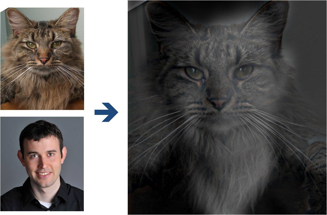
(Look at image on right from very close, then from far away.)
Overview
The goal of this part of the assignment is to create hybrid images using the approach
described in the SIGGRAPH 2006 paper
by Oliva, Torralba, and Schyns. Hybrid images are static images that
change in interpretation as a function of the viewing distance. The basic idea is that high frequency tends
to dominate perception when it is available, but, at a distance, only the low
frequency (smooth) part of the signal can be seen. By blending the high frequency portion of one image with the low-frequency portion of another, you get a hybrid image that leads to different interpretations at different distances.
Details
Here, we have included two sample images (of Derek and his former cat Nutmeg) and some matlab
starter code that can be used to load two images and align them. Here is the python version. The alignment is important because it affects
the perceptual grouping (read the paper for details).
-
First, you'll need to get a few pairs of images that you want to make into
hybrid images. You can use the sample
images for debugging, but you should use your own images in your results. Then, you will need to write code to low-pass
filter one image, high-pass filter the second image, and add (or average) the
two images. For a low-pass filter, Oliva et al. suggest using a standard 2D Gaussian filter. For a high-pass filter, they suggest using
the impulse filter minus the Gaussian filter (which can be computed by subtracting the Gaussian-filtered image from the original).
The cutoff-frequency of
each filter should be chosen with some experimentation.
- For your favorite result, you should also illustrate the process through frequency analysis. Show the log magnitude of the Fourier transform of the two input images, the filtered images, and the
hybrid image. In MATLAB, you can compute and display the 2D Fourier transform with
with:
imagesc(log(abs(fftshift(fft2(gray_image)))))and in Python it's plt.imshow(np.log(np.abs(np.fft.fftshift(np.fft.fft2(gray_image)))))
- Try creating a variety of types of hybrid images (change of expression,
morph between different objects, change over time, etc.).
Bells & Whistles (Extra Points)
Try using color to enhance the effect.
Does it work better to use color for the high-frequency component, the
low-frequency component, or both? (2 points)
Part 1.3: Gaussian and Laplacian Stacks
Overview
In this part you will implement Gaussian and Laplacian stacks, which are kind of like pyramids but without the downsampling. Then you will use these to analyze some images, and your results from part 1.2.
Details
-
Implement a Gaussian and a Laplacian stack. The different between a stack and a pyramid is that in each level of the pyramid the image is downsampled, so that the result gets smaller and smaller.
In a stack the images are never downsampled so the results are all the same dimension as the original image, and can all be saved in one 3D matrix (if the original image was a grayscale image).
To create the successive levels of the Gaussian Stack, just apply the Gaussian filter at each level, but do not subsample.
In this way we will get a stack that behaves similarly to a pyramid that was downsampled to half its size at each level. If you would rather work with pyramids, you may implement pyramids other than stacks. However, in any case, you are NOT allowed to use matlab's impyramid() and its equivalents in this project. You must implement your stacks from scratch!
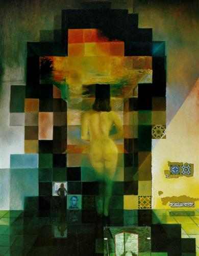
- Apply your Gaussian and Laplacian stacks to interesting images that contain structure in multiple resolution such as paintings like the Salvador Dali painting of Lincoln and Gala we saw in class, or the Mona Lisa. Display your stacks computed from these images to discover the structure at each resolution.
- Illustrate the process you took to create your hybrid images in part 1 by applying your Gaussian and Laplacian stacks and displaying them for your favorite result. This should look similar to Figure 7 in the Oliva et al. paper.
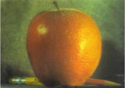
Part 1.4: Multiresolution Blending (a.k.a. the oraple!)
Overview
The goal of this part of the assignment is to blend two images seamlessly using a multi resolution blending as described in the 1983 paper by Burt and Adelson. An image spline is a smooth seam joining two image together by gently distorting them. Multiresolution blending computes a gentle seam between the two images seperately at each band of image frequencies, resulting in a much smoother seam.
Details
Here, we have included the two sample images from the paper (of an apple and an orange).
- First, you'll need to get a few pairs of images that you want blend together with a vertical or horizontal seam. You can use the sample
images for debugging, but you should use your own images in your results. Then you will need to write some code in order to use your Gaussian and Laplacian stacks from part 2 in order to blend the images together. Since we are using stacks instead of pyramids like in the paper, the algorithm described on page 226 will not work as-is. If you try it out, you will find that you end up with a very clear seam between the apple and the orange since in the pyramid case the downsampling/blurring/upsampling hoopla ends up blurring the abrupt seam proposed in this algorithm. Instead, you should always use a mask as is proposed in the algorithm on page 230,
and remember to create a Gaussian stack for your mask image as well as for the two input images. The Gaussian blurring of the mask in the pyramid will smooth out the transition between the two images. For the vertical or horizontal seam, your mask will simply be a step function of the same size as the original images.
- Now that you've made yourself an oraple (a.k.a your vertical or horizontal seam is nicely working), pick a couple of images to blend together with an irregular mask, as is demonstrated in figure 8 in the paper.
- Blend together some crazy ideas of your own!
- Illustrate the process by applying your Laplacian stack and displaying it for your favorite result and the masked input images that created it. This should look similar to Figure 10 in the paper.
Bells & Whistles (Extra Points)
- Try using color to enhance the effect. (2 points)
Part 2: Gradient Domain Fushion
Overview
This project explores gradient-domain processing, a simple technique
with a broad set of applications including blending, tone-mapping, and
non-photorealistic rendering. For the core project, we will focus on
"Poisson blending"; tone-mapping and NPR can be investigated as bells
and whistles.
The primary goal of this assignment is to
seamlessly blend an object or texture from a source image into a
target image. The simplest method would be to just copy and paste the
pixels from one image directly into the other. Unfortunately, this
will create very noticeable seams, even if the backgrounds are
well-matched. How can we get rid of these seams without doing too
much perceptual damage to the source region?
One way to approach this is to use the Laplacian pyramid blending technique we implemented for the last project (and you will compare your new results to the one you got from Laplacian blending). Here we take a different approach. The insight we will use is
that people often care much more about the gradient of an image than
the overall intensity. So we can set up the problem as finding values
for the target pixels that maximally preserve the gradient of the
source region without changing any of the background pixels. Note
that we are making a deliberate decision here to ignore the overall
intensity! So a green hat could turn red, but it will still look like
a hat.
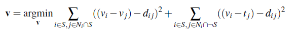
We can formulate our objective as a least squares
problem. Given the pixel intensities of the source image "s" and of
the target image "t", we want to solve for new intensity values "v"
within the source region "S":

Here, each "i" is a pixel in the source region "S",
and each "j" is a 4-neighbor of "i". Each summation guides the
gradient values to match those of the source region. In the first
summation, the gradient is over two variable pixels; in the second,
one pixel is variable and one is in the fixed target region.
The method presented above is called "Poisson blending". Check out the Perez et al. 2003 paper to see sample results, or to wallow in extraneous math. This is just one example of a more general set of gradient-domain processing techniques. The general idea is to create an image by solving for specified pixel intensities and gradients.
A Wordy Explanation
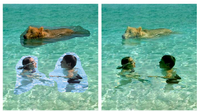 As an example, consider this picture of the bear and swimmers being pasted into a pool of water. Let's ignore the bear for a moment and consider the swimmers. In the above notation, the source image "s" is the original image the swimmers were cut out of; that image isn't even shown, because we are only interested in the cut-out of the swimmers, i.e., the region "S". "S" includes the swimmers and a bit of light blue background. You can clearly see the region "S" in the left image, as the cutout blends very poorly into the pool of water. The pool of water, before things were rudely pasted into it, is the target image "t".
So, how do we blend in the swimmers? We construct a new image "v" whose gradients inside the region "S" are similar to the gradients of the cutout we're trying to paste in (swimmers + a little bit of background). The gradients won't end up matching exactly: the least squares solver will take any hard edges of the cutout at the boundary and smooth them by spreading the error over the gradients inside "S".
Outside "S", "v" will match the pool. We won't even bother computing the gradients of the pool outside S; we'll just copy those pixels directly.
In the first half of the large equation above, we set the gradients of "v" inside S. We loop over all the pixels inside the region S, and request that our new image "v" have the same gradients as the swimmers. The summation is over every pixel i in S; j is the 4 neighbors of i (left, right, up, and down, giving us both the x and y gradients. You may notice this equation counts all the gradients twice - is was simpler to write it this way. You actually don't have to double-count everything; it doesn't affect the result.)
But what do we do around the boundary of "S"? I.e. what if i is inside S, but j is outside? That's the second half of the equation. (If you look closely at the variables under the summation sign, the S has a bar thing in front of it - that means the complement of S, or anything not in S. Thus, read "j in the 4-neighborhood of i, but j not in S"). In this case we aren't solving for a v_j, since j is not inside "S". So we just pluck the intensity value right out of the target image. Thus we use t_j. Remember, we aren't modifying t outside the area of S, so we know that v_j in this case isn't a variable: it's exactly equal to t_j.
Part 2.1 Toy Problem (10 pts)
 The implementation for gradient domain processing is not complicated, but it is easy to make a mistake, so let's start with a toy example. In this example we'll compute the x and y gradients from an image s, then use all the gradients, plus one pixel intensity, to reconstruct an image v.
Denote the intensity of the source image at (x, y) as s(x,y) and the values of the image to solve for as v(x,y). For each pixel, then, we have two objectives:
| 1. | minimize ( v(x+1,y)-v(x,y) - (s(x+1,y)-s(x,y)) )^2 | the x-gradients of v should closely match the x-gradients of s |
| 2. | minimize ( v(x,y+1)-v(x,y) - (s(x,y+1)-s(x,y)) )^2 | the y-gradients of v should closely match the y-gradients of s |
Note that these could be solved while adding any constant value to v, so we will add one more objective:
| 3. | minimize (v(1,1)-s(1,1))^2 | The top left corners of the two images should be the same color |
For 10 points, solve this optimization as a least squares problem. If your solution is correct, then you should recover the original image.
Implementation Details
The first step is to write the objective function as a set of least squares constraints in the standard matrix form: (Av-b)^2. Here, "A" is a sparse matrix, "v" are the variables to be solved, and "b" is a known vector. It is helpful to keep a matrix "im2var" that maps each pixel to a variable number, such as:
[imh, imw, nb] = size(im);
im2var = zeros(imh, imw);
im2var(1:imh*imw) = 1:imh*imw;
(If you find that matlab trickery confusing, understand that you could have performed the mapping between pixel and variable number manually each time: e.g. the pixel at s(r,c), uses the variable number (c-1)*imh+r. However, this trick will come in handy for Poisson blending, where the mapping is from an arbitrarily-shaped block of pixels and won't be such a simple function. So it makes sense to understand it now.)
Then, you can write Objective 1 above as:
e=e+1;
A(e, im2var(y,x+1))=1;
A(e, im2var(y,x))=-1;
b(e) = s(y,x+1)-s(y,x);
Here, "e" is used as an equation counter. Note that the y-coordinate is the first index in Matlab convention. Objective 2 is similar; add all the y-gradient constraints as more rows to the same matrices A and b.
As another example, Objective 3 above can be written as:
e=e+1;
A(e, im2var(1,1))=1;
b(e)=s(1,1);
To solve for v, use
v = A\b; or
v = lscov(A, b);
Then, copy each solved value to the appropriate pixel in the output image.
Part 2.2 Poisson Blending (30 pts)
Step 1: Select
source and target regions. Select the boundaries of a region in the
source image and specify a location in the target image where it
should be blended. Then, transform (e.g., translate) the source image
so that indices of pixels in the source and target regions correspond.
I've provided starter code
(getMask.m, alignSource.m) to help with this. In case you are using python, Nikhil Shinde who took the course in 2018 provided a starter code that will produce a mask for you. You may want to augment
the code to allow rotation or resizing into the target region. You
can be a bit sloppy about selecting the source region -- just make
sure that the entire object is contained. Ideally, the background of
the object in the source region and the surrounding area of the target
region will be of similar color.
Step 2: Solve the blending
constraints:
Step 3: Copy the solved values v_i into your target image. For RGB
images, process each channel separately. Show at least three results
of Poisson blending. Explain any failure cases (e.g., weird colors,
blurred boundaries, etc.).
Tips
1. Pre-initialize your sparse matrix with
sparse([], [], [], M, N, nzmax)
for a matrix with M equations and N variables and at most nzmax non-zero entries.
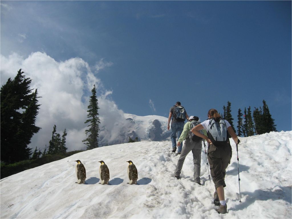
2. For your first blending example, try something that you know should work, such as the included penguins on top of the snow in the hiking image.
3. Object region selection can be done very crudely, with lots of room around the object.
Bells & Whistles (Extra Points)
Mixed Gradients (5 pts)
Follow the same steps as Poisson blending, but use the gradient in source or target with the larger magnitude as the guide, rather than the source gradient:
Here "d_ij" is the value of the gradient from the source or the target image with larger magnitude, i.e. if abs(s_i-s_j) > abs(t_i-t_j), then d_ij = s_i-s_j; else d_ij = t_i-t_j. Show at least one result of blending using mixed gradients. One possibility is to blend a picture of writing on a plain background onto another image.
Color2Gray (2 pts)
Sometimes, in converting a color image to grayscale (e.g., when printing to a laser printer), we lose the important contrast information, making the image difficult to understand. For example, compare the color version of the image on right with its grayscale version produced by rgb2gray.
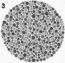
Can you do better than rgb2gray? Gradient-domain processing provides one avenue: create a gray image that has similar intensity to the rgb2gray output but has similar contrast to the original RGB image. This is an example of a tone-mapping problem, conceptually similar to that of converting HDR images to RGB displays. To get credit for this, show the grayscale image that you produce (the numbers should be easily readable).
Hint: Try converting the image to HSV space and looking at the gradients in each channel. Then, approach it as a mixed gradients problem where you also want to preserve the grayscale intensity.
More gradient domain processing (up to 3 pts)
Many other applications are possible, including non-photorealistic rendering, edge enhancement, and texture or color transfer. See Perez et al. 2003 and GradientShop for further ideas.
Materials
- Images, including the toy image, sample images for blending, and the color2gray image.
- Starter Code, including a top-level script and functions to select the source region and align source and target images for blending. Python starter code by Nikhil Shinde.
Deliverables
Use both words and images to show us what you've done (describe in detail your algorithm parameterization for each of your results).
Submit all code to bCourses. Make sure each part of the project has a main.m or main.py file that can execute that part of the assignment in full and include a README describing the contents of each file.
In the website in your uploaded directory, please:
The first part of the assignment is worth 50 points, as follows:
- 20 points for the implementation of all four parts of the project.
- The following are the points for the project html page description as well as results:
3 points for the warmup: Show us your sharpened image, including the original one.
5 points for hybrid images and the Fourier analysis;
5 points for including at least two hybrid image examples beyond the first (including at least one failure);
10 points for multiresolution blending;
5 points for including at least two multiresolution blending examples beyond the apple+orange,
one of them with an irregular mask.
2 points for clarity.
The second part of the assignment is worth 50 points, as follows:
- (10 points) Include a brief description of the project.
- (10 points) Finish the toy problem.
- (10 points) Show your favorite blending result. Include: 1) the source and target image; 2) the blended image with the source pixels directly copied into the target region; 3) the final blend result. Briefly explain how it works, along with anything special that you did or tried. This should be with your own images, not the included samples.
- (10 points) Next, show at least two more results for Poisson blending, including one that doesn't work so well (failure example). Explain any difficulties and possible reasons for bad results.
- (10 points) Choose one pair of images that you blended together using Laplacian pyramid blending in the part 1 and now blend it using the Poisson blending techniques. Display the original images as well as the different blending results (i.e. Laplacian pyramid blending, Poisson Image Blending, Mixed graident blending (If you do the B & W)). Which approach works best for these images? Why? When do you think that one approach would be more appropriate than another?
For this project, you can also earn up to 10 extra points for the bells & whistles mentioned above
or suggest your own extensions (check with prof first).
Tell us about the most important thing you learned from this project!
Acknowledgements
The hybrid images part of this assignment is borrowed
from Derek Hoiem's
Computational Photography class.
This gradient domain part of this assignment was based on one offered by Derek Hoiem.
Here is another description of it from James Hays.
 Programming Project #3 (proj3)