Overview
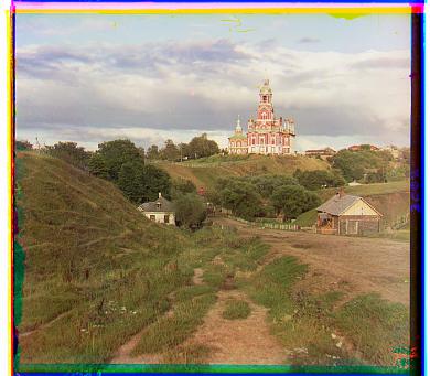
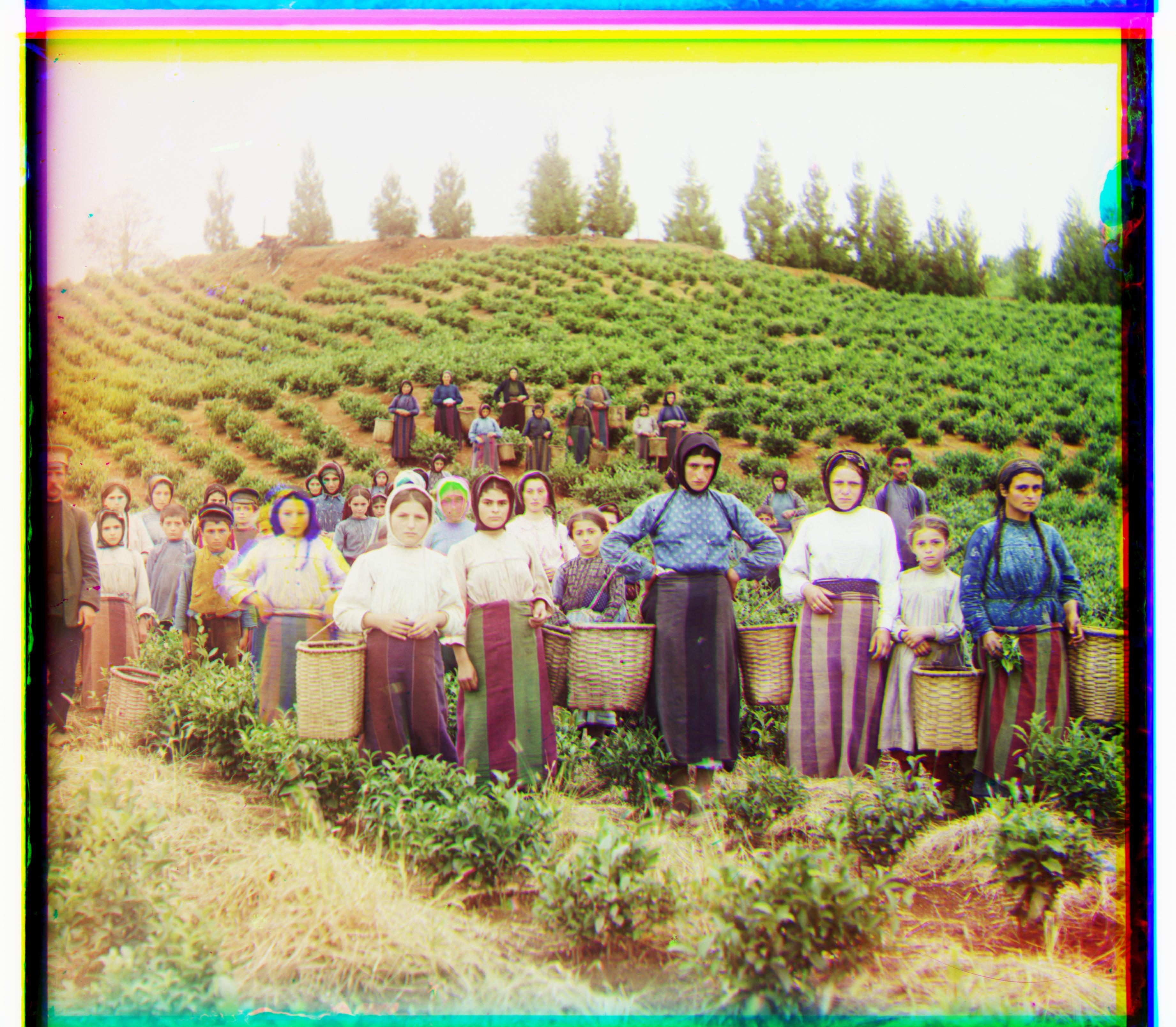
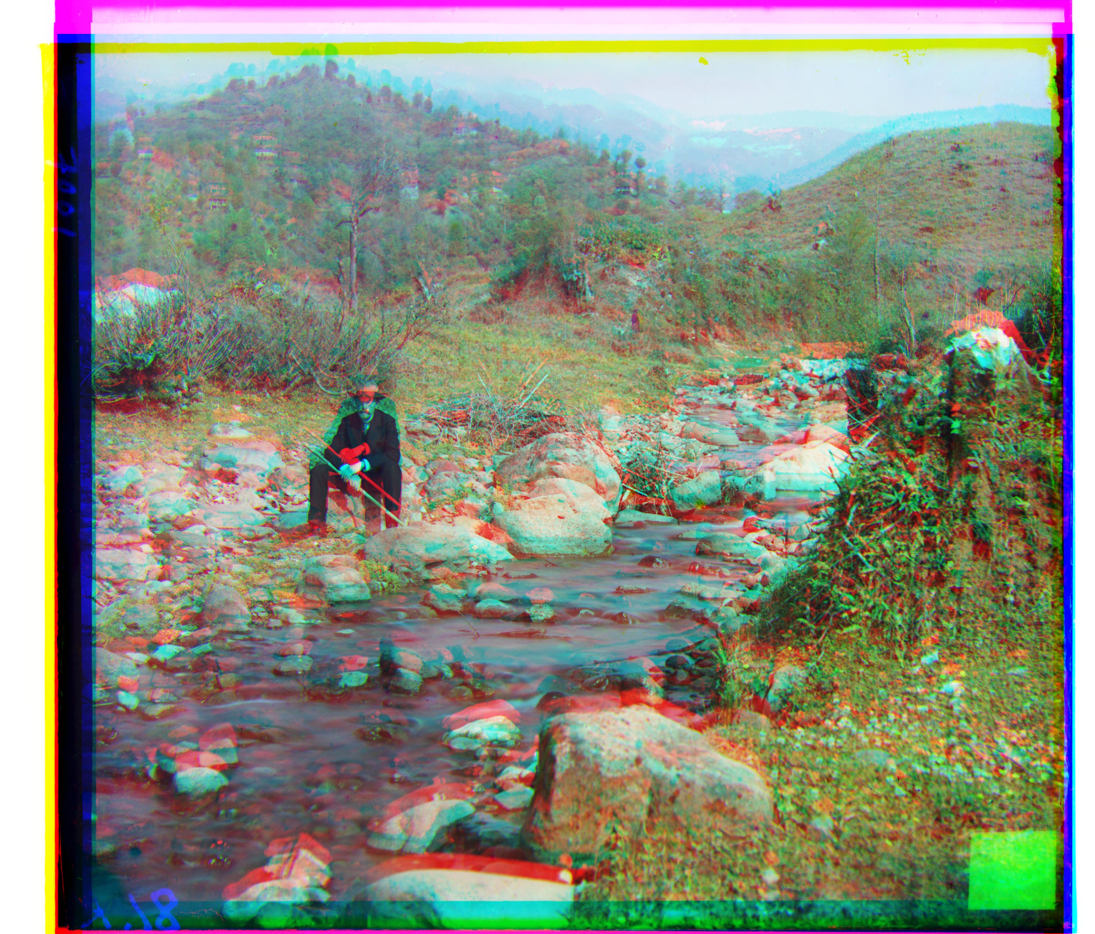
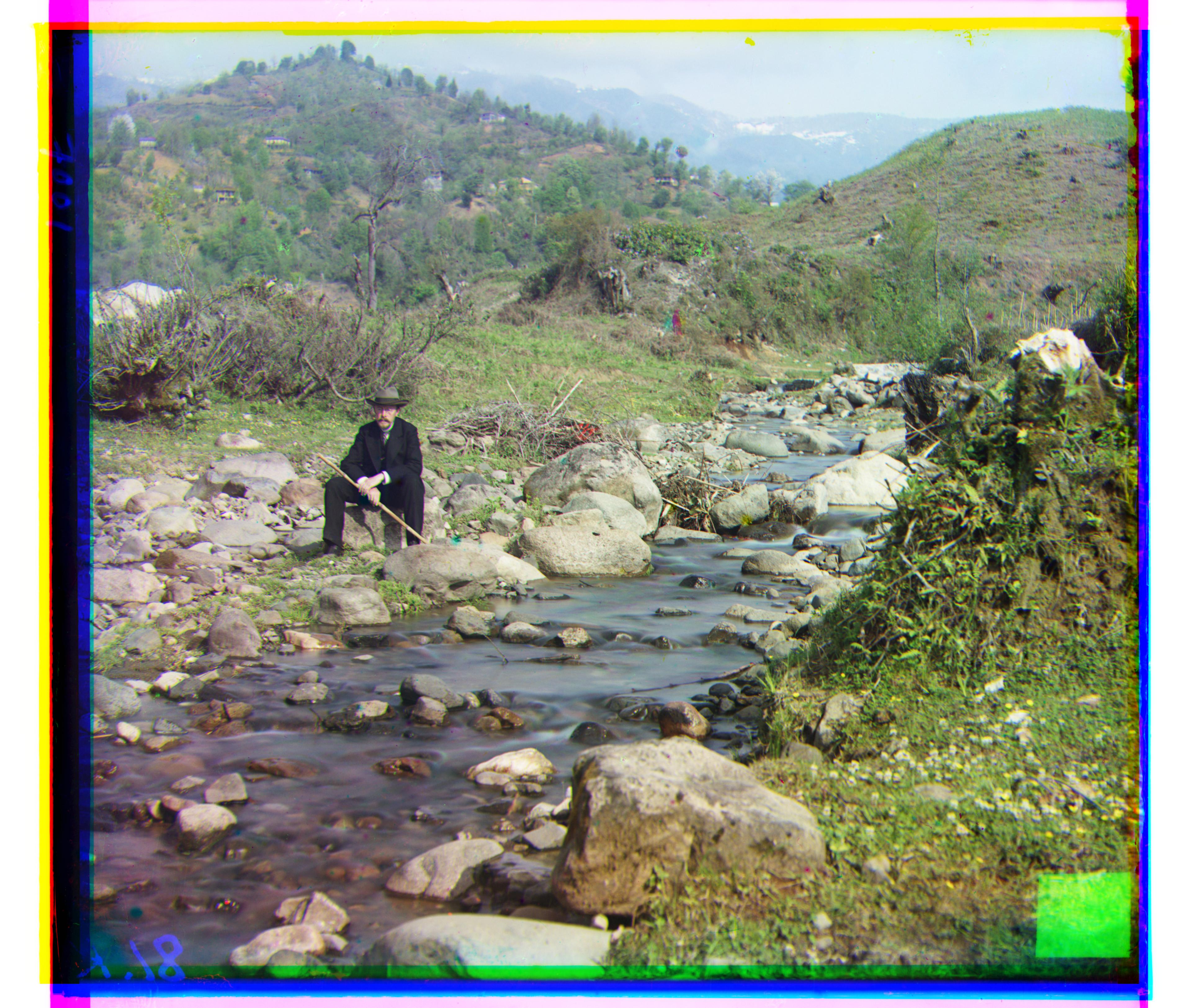
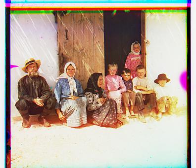
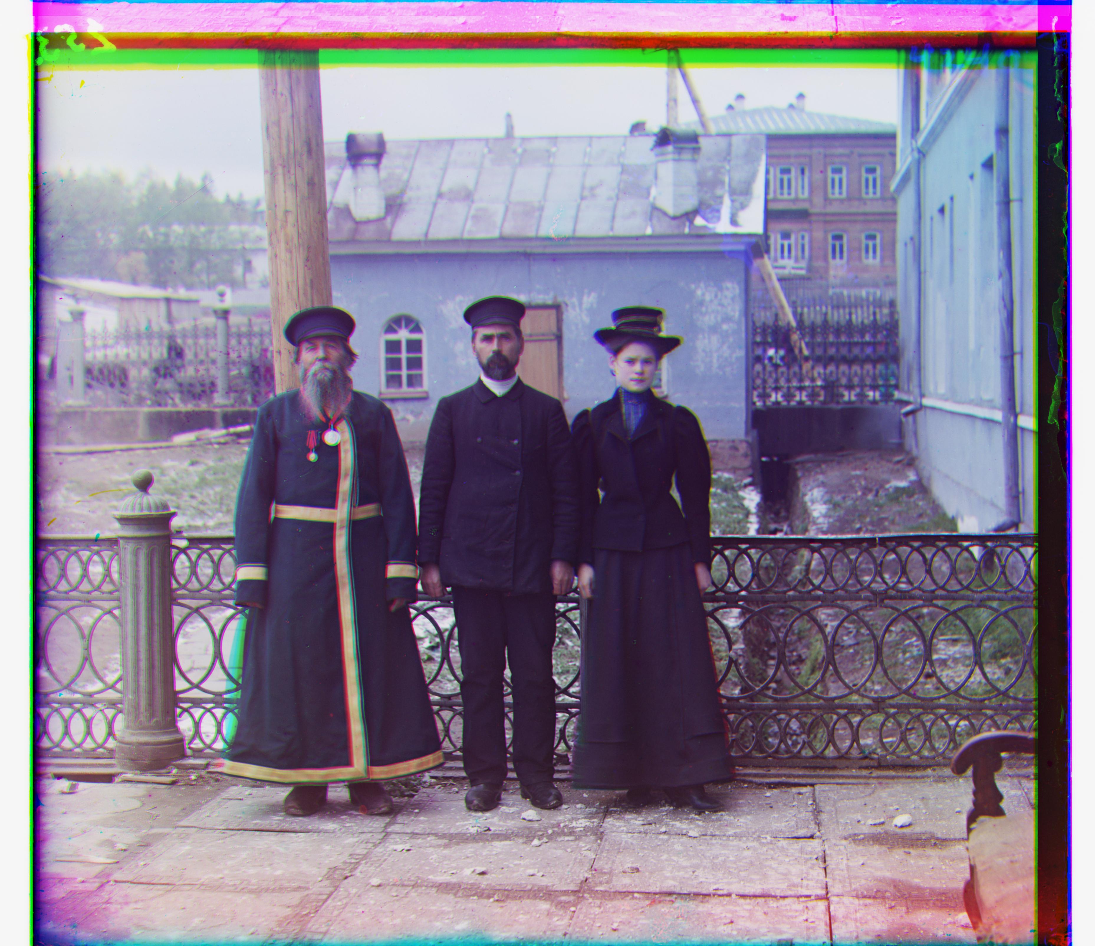
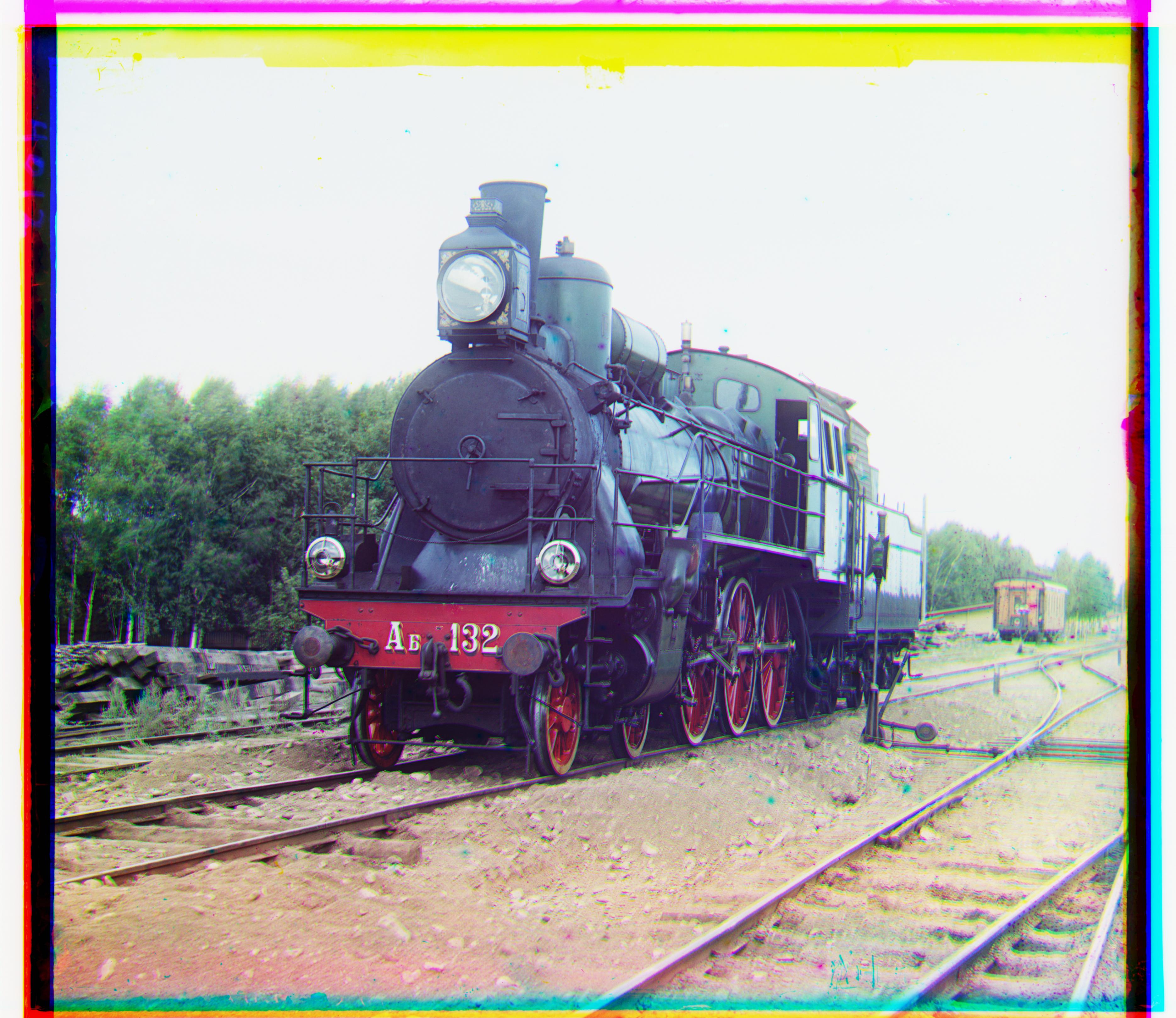
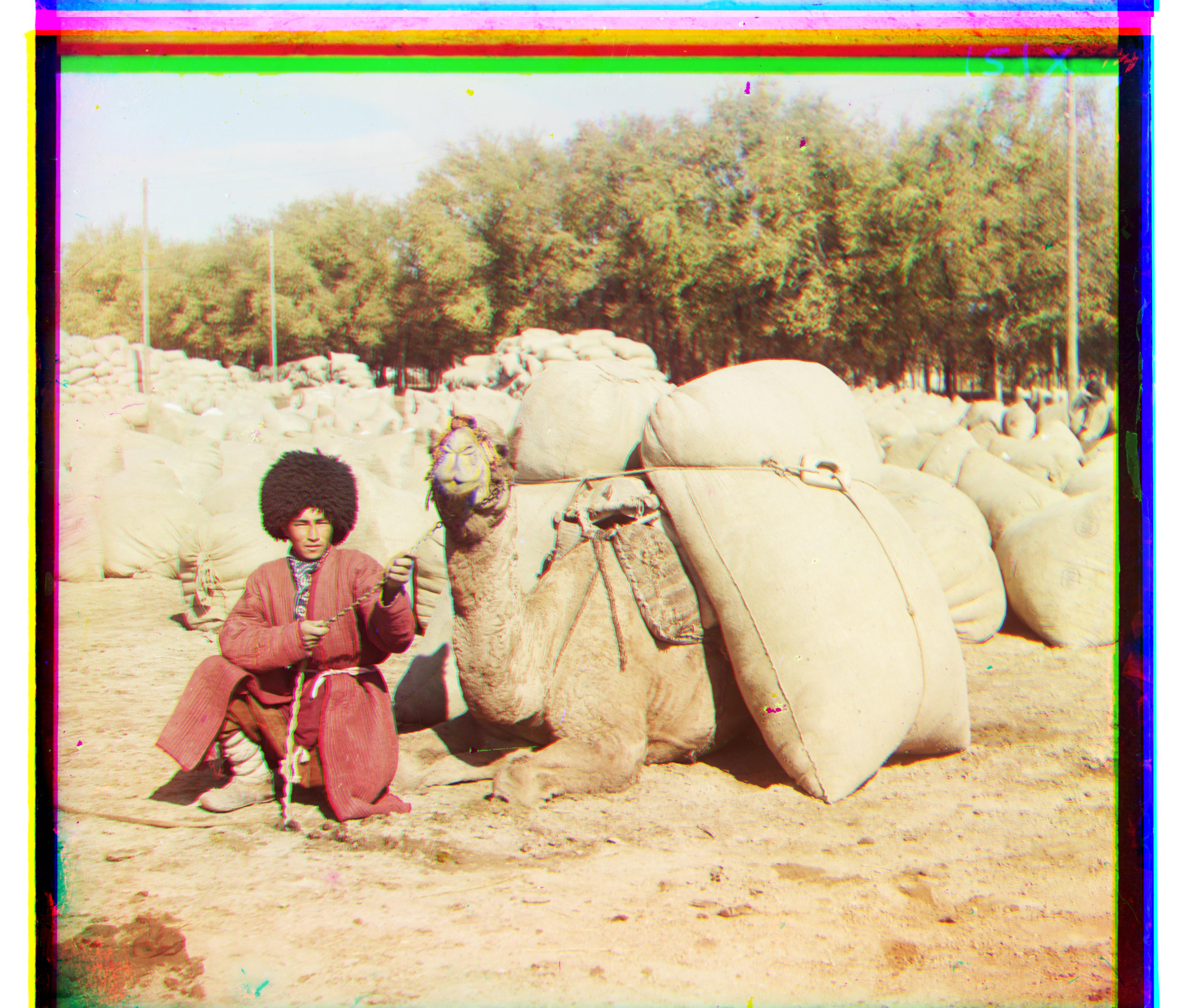
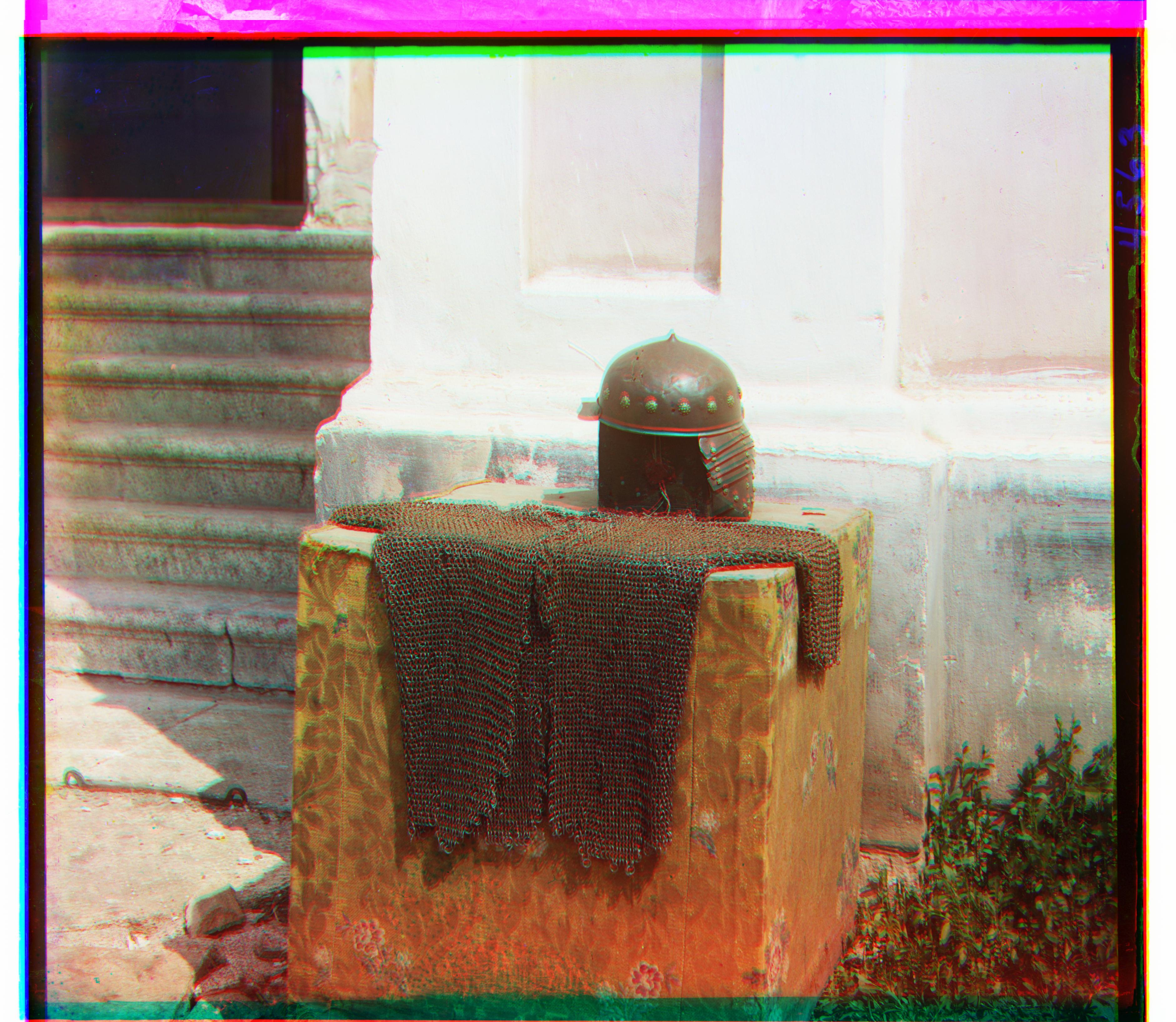
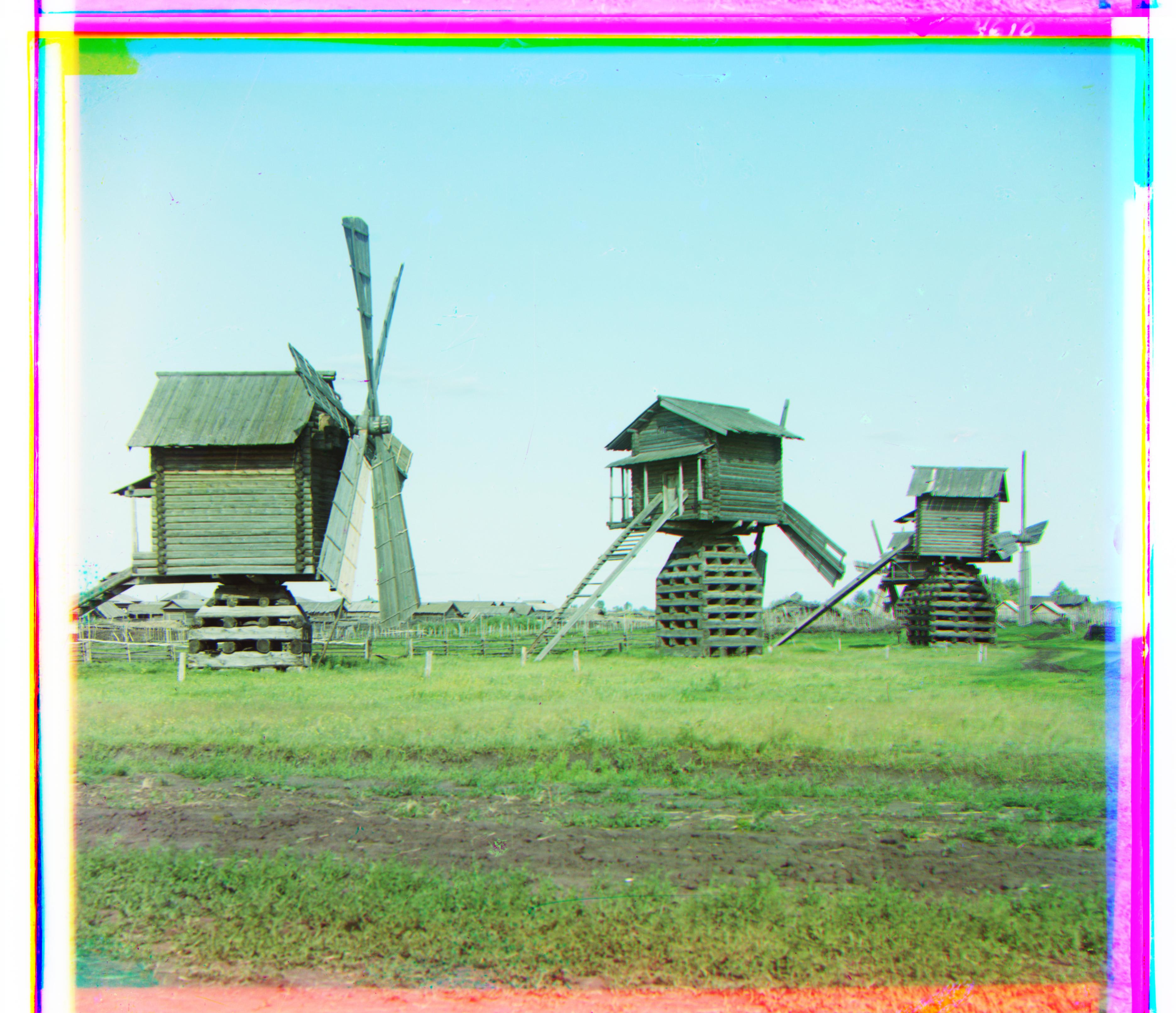
The Prokudin-Gorskii photo collection provides us a rare and vivid look at the early 20th century but it takes a bit of work to get there. Each photograph is a set of three exposures, capturing the scene in red, green and blue. To produce a color image, these recorded exposures needed to be overlaid onto each other using a special projector. These projectors were never made so these pictures remained in black & white for years until acquired by the Library of Congress in 1948. Now that Prokudin-Gorskii collection has been digitized and made available for the public, we can colorize these photos ourselves by processing and aligning the channels on top of each other!
Algorithm
Single-Scale Alignment
The processing begins with the digitized glass plate, which contains the red, green, and blue exposures. This image is divided vertically into equal thirds so we can analyze each color channel individually. A generic crop trims the images by 15% on all sides. This is to remove picture borders and other prominent edge discolorings during the calculations. The blue channel is treated as the "base" channel, so the goal is to align the red and green channels in a way that best matches the blue channel. A matching score is calculated by accumulating the Sum of Squared Differences (SSD) distance against the stationary blue channel with a pixel-shifted red/green channel. The process is run with a pixel shifting window of [-15, 15], meaning the red/green channel has its pixels shifted by its x-axis and y-axis a total of 31 x 31 times. Since the more alike the brightness of the pixels for the red/green channel is to the blue indicates a better match, the lowest score is selected from these entries. The ideal displacement vector is retrieved in the form (x, y). The original divided green and red channels are then shifted by their respective displacement vectors. The now-shifted channels are compiled to produce a color image.
Multi-Scale Alignment
An exhaustive search is manageable with images that have small pixels count, but the collection is available to download in a high quality .tif format. To expedite our processing, an "image pyramid" search is needed. The large image is repeatedly resized to be half its size until it reaches a minimum of 400 x 400. At this point of single-scale alignment is run, returning a red and green displacement vector. This vector is doubled in proportion with the image until the image reaches its initial size again. The displacement vectors are applied to the red and green channels. Correction vectors are then calculated by running the single-scale alignment with a window of [-2, 2] on the newly aligned channels. Once these correction vectors are applied, the channels are compiled to produce a color image.
Problems
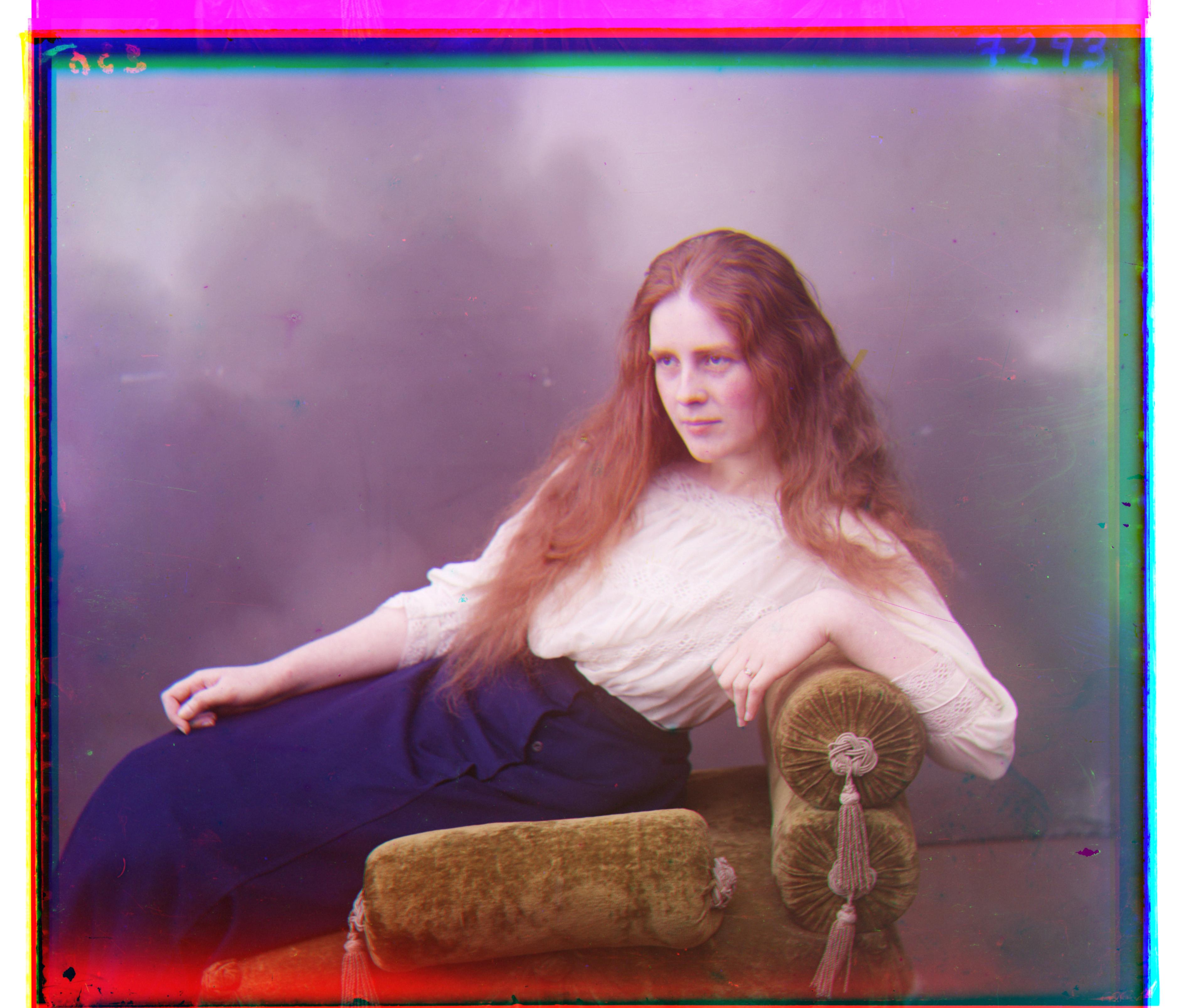
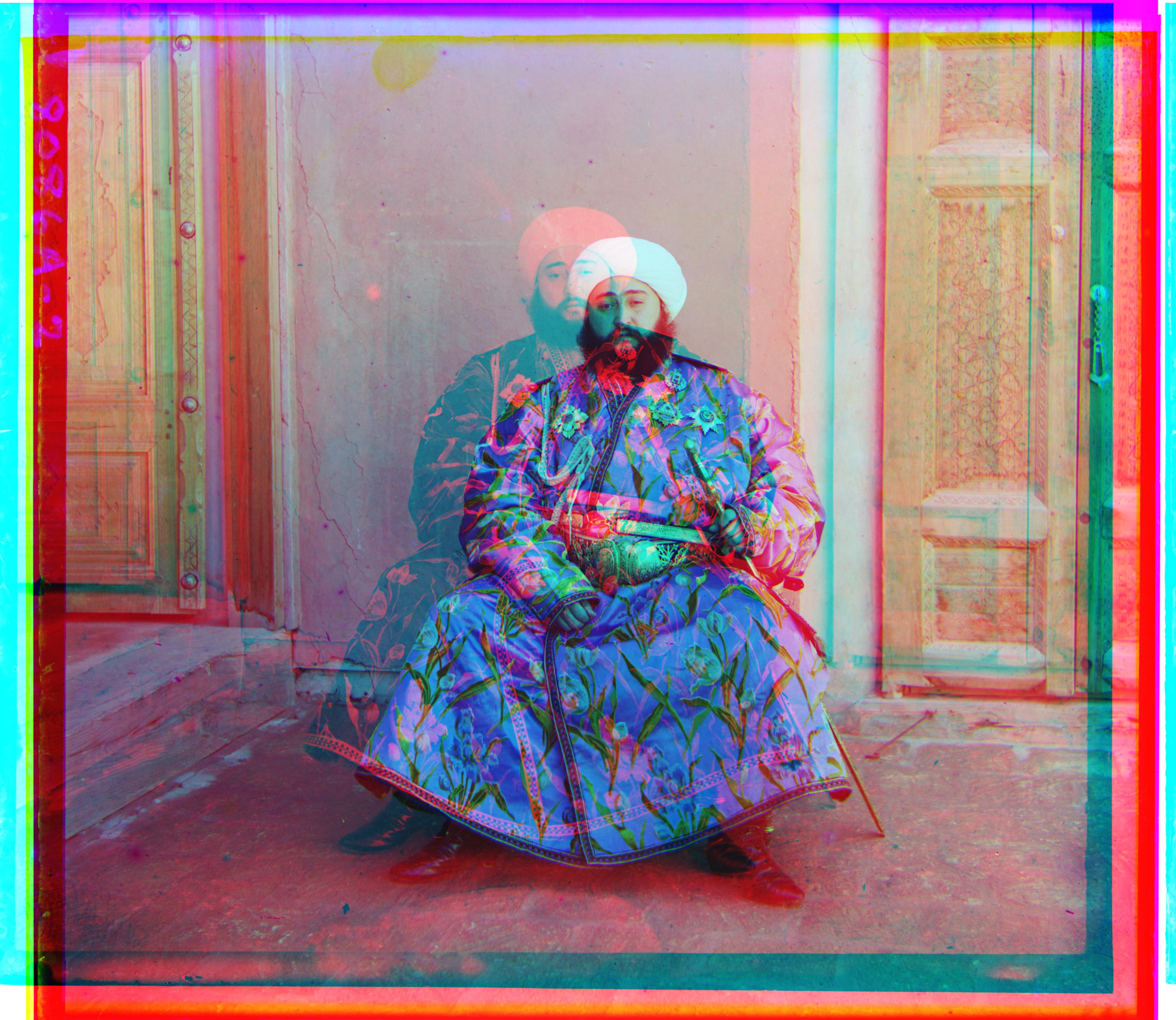
I had some trouble optimizing my SSD calculation. I mistakenly used a nested list comprehension which calculated and assigned each SSD score in a wasteful fashion. Taking advantage of np.sum and np.subtract sped up my implementation considerably. A small .jpg image took an average of 40 seconds to run on my old implementation but now takes around 3 seconds. I also had trouble with self_portrait.tif, which failed to align properly on both my greyscale and canny edge implementations. Getting this image to align using the red and blue channels produced a more acceptable result.
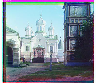
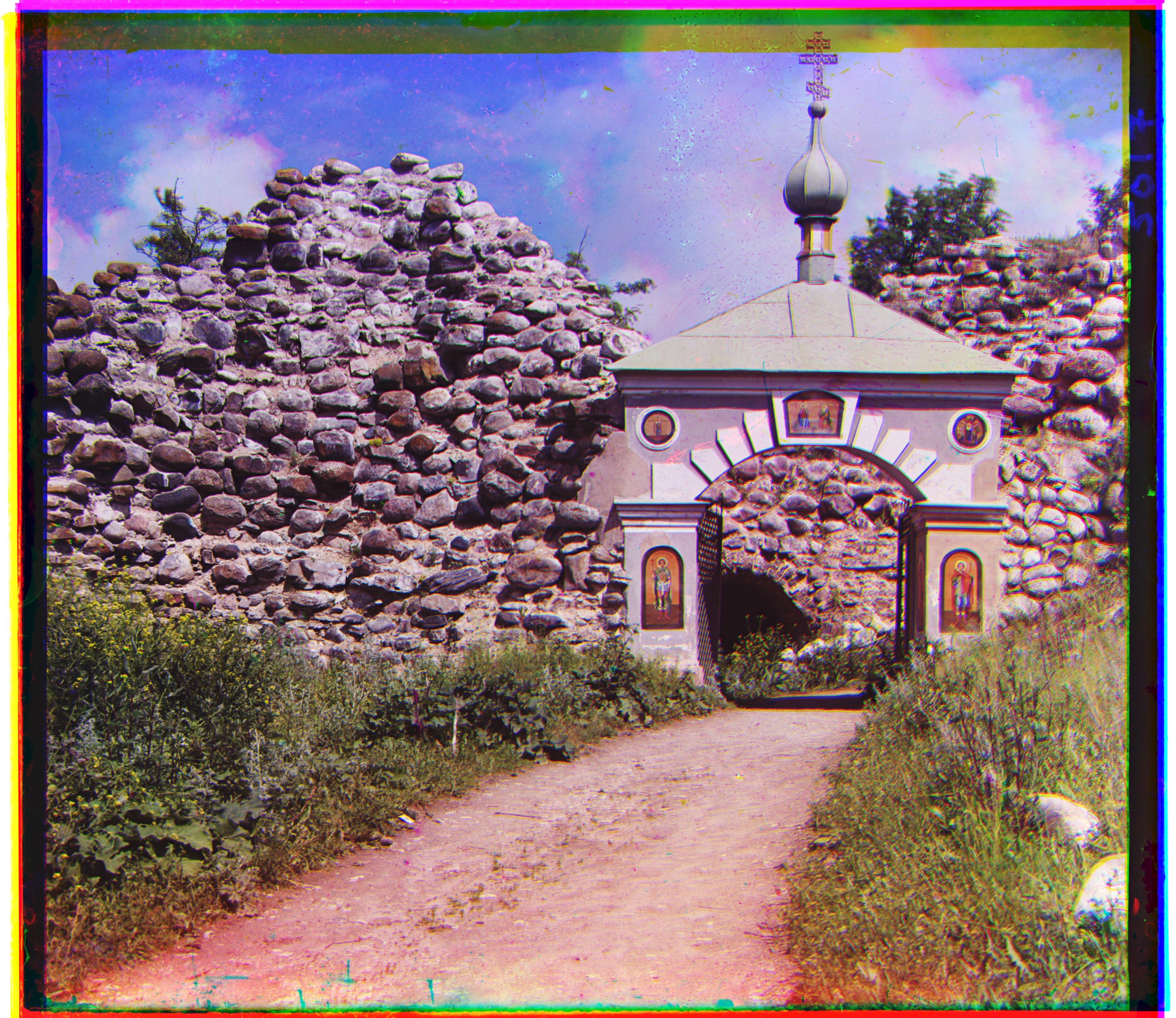
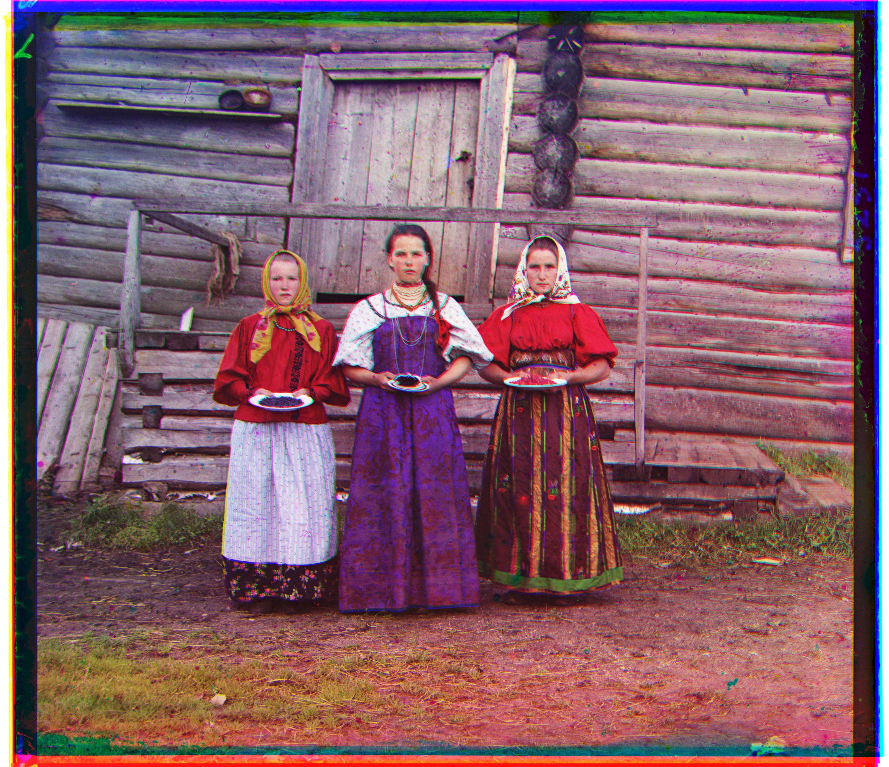
Example Images
|

|
|
|
|

|
|
|
|
|
|
|

|
|
Selected Pictures from the Collection
|
|
|
|
Bells & Whistles
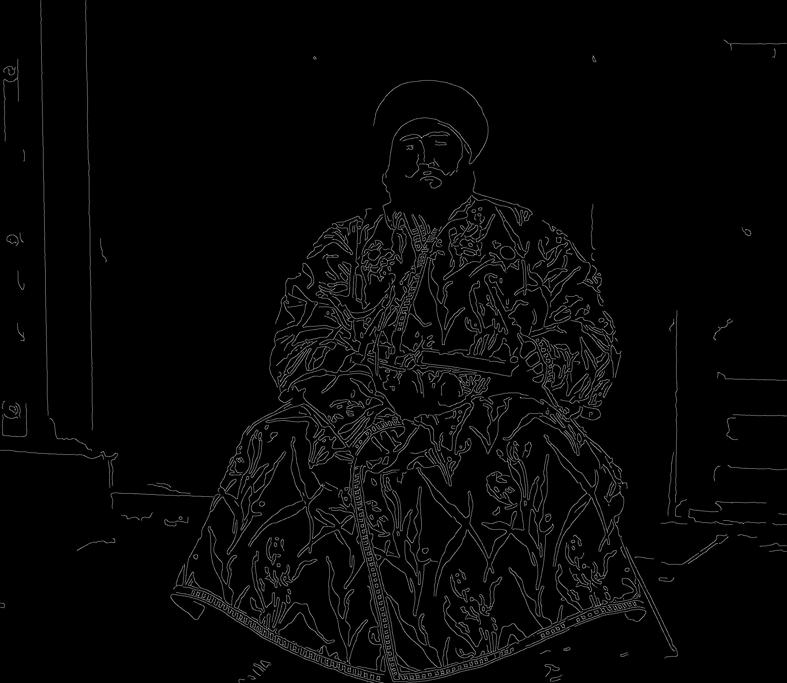
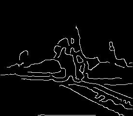
Canny Edge Detection
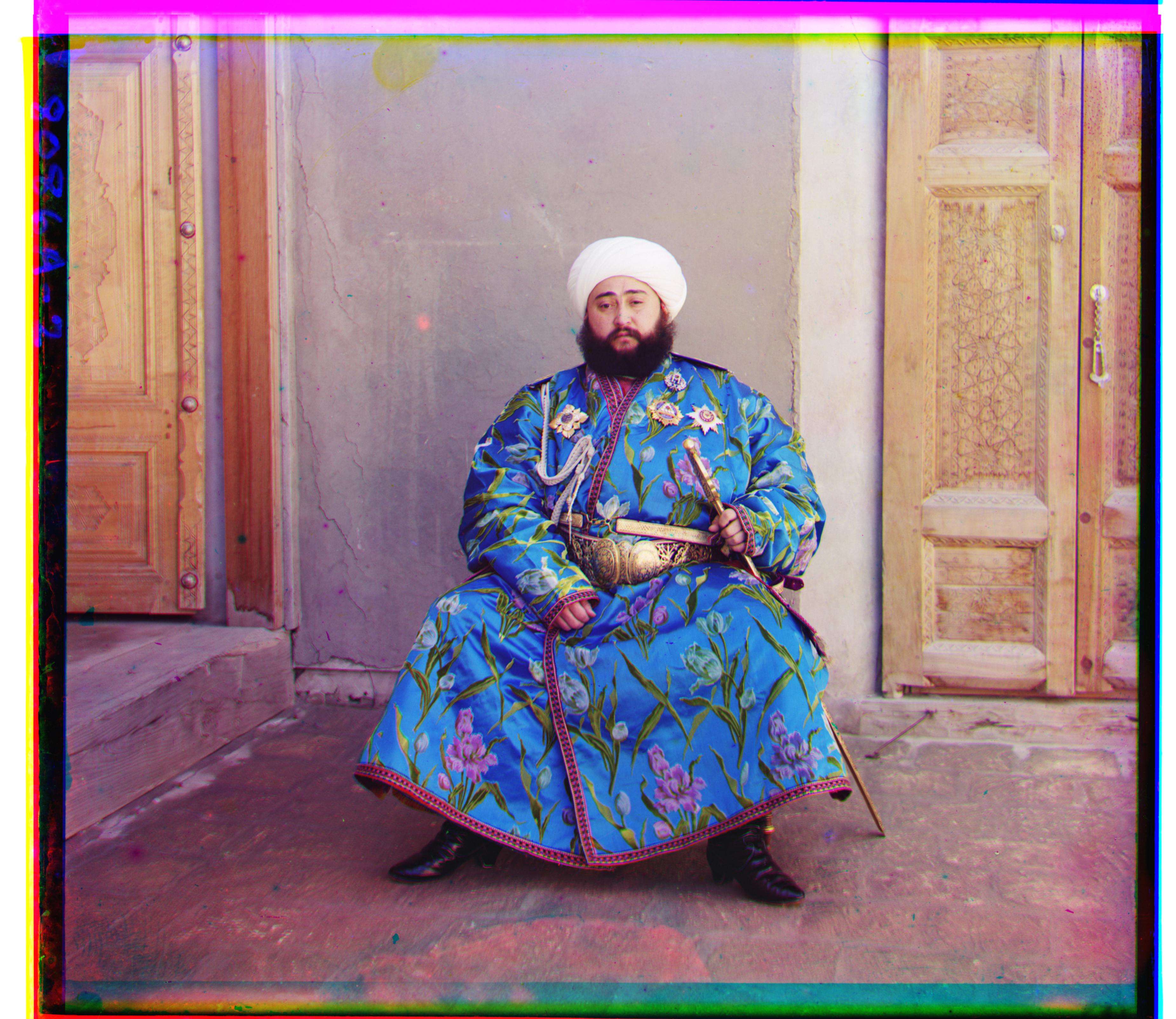
To improve the accuracy of the SSD calculations, canny edge detection (with an sigma value of 3) was implemented. The cropped images are converted to "outline" variants by running a filter that detects and isolates edges. By emphasizing the prominent shapes and contours of the image, alignments were generally more accurate. Noise that misled the calculations of the greyscale SSD calculations would not be present when working with edge variants. Most of the example images above were calculated with Canny Edge detection. The exceptions were for the smaller .jpg images for which the displacements vectors were occasionaly off by 1. A working theory for this is that, much like borders and discolorations, the "outline" versions inflate the ssd scores for the alignments that would normally work.
|
|
|
|
|
|
|
|
|
|