Project 1: Colorizing the Prokudin-Gorskii Photo Collection

In this project, I explored numerous computational photography techniques to colorize the photos in the Prokudin-Gorskii collection, each of which contains three image plates captured using a blue filter, green filter, and a red filter.

The deliverables are: an efficient edge-based aligning algorithm for colorization, a re-mapping of the RGB color space for the digital negatives, and a simple color balancing as post-process.

Alignment

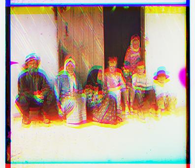
Simply separate the digital negatives to three equal parts will get unaligned images. Here are two examples:

Basic Idea
Assume we only have vertical and/or horizontal displacement between the images. We can shift the values in the image 2darray by using np.roll to get the transformed image. We need to determine the displcement (x_shift, y_shift) on a search_image which yields the best matching results on the base_image. I followed the advice from our TA - align blue and red channel against the green channel. And my experiment also revealed aligning against blue/red channel produces less accurate results.
In my algorithm, the matching function is the normalized cross-correlation (NCC) between search_image and base_image. It's the inner product of two normalized vectors, which is widely used to find the degree of similarity between two signals. I also tried sum of squared difference (SSD) as the matching indicator but the results were less satisfactory.
left: SSD + Align against Blue ; right: NCC + Align against Green

Exhaustive Search
Initially, my implementation for the aforementioned idea consists of simple nested for-loop, which shifts the image by a range of [-15, 15]. It returns the displacement which yields the highest NCC. For the small-sized .jpg image, the algorithm finishes within 0.5 sec. However, for the .tif image, the average runtime is about 4-5 minutes.
Course-to-fine Search
To make the algorithm faster, we can first do search on the down-sampled search_image and base_image. The function works in a recursive manner, with the base case being if the down-sampled image reaches the thumbnail-size about 300px * 300px, return the shift offsets found using the naive search. The recursive step will find the best (x_shift, y_shift) on a smaller image whose size is halved. Then, we can start searching the offsets for this level starting from (x_shift, y_shift) with displacements with a range of [0, 3].
This image pyramids search can return the offsets for big .tif images within 20 sec.
(BELLS & WHISTLES) Edge Alignment
Lastly, I experimented with the Canny edge detector to extract contours. Using them as alignment baseline produces slightly better results compared with the bare intensity values since fundamentally the edges define the shape. With the help of the edge detector, we achieved very satisfactory alignment for emir.tif.
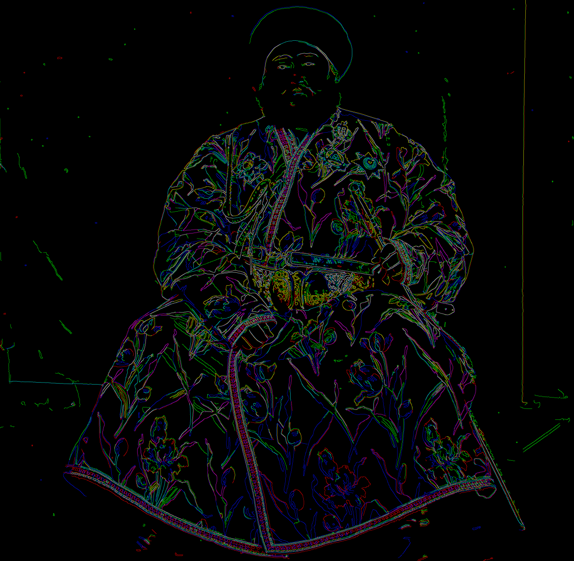
However, There are still some misalignments, as you can see in the close-up edge-matching image. They are probably introduced by other transformations such as rotations and scaling which we did not take account of. Adding these transformations into the search algorithm can be one of the future works.

(BELLS & WHISTLES) Color Space Remapping

Basic Idea
There is no reason to assume that the red, green, and blue lenses used by Produkin-Gorskii correspond directly to the R, G, and B channels in the digital RGB color space. Based on a "ground-truth" image, I managed to find a mapping that produces more realistic colors.
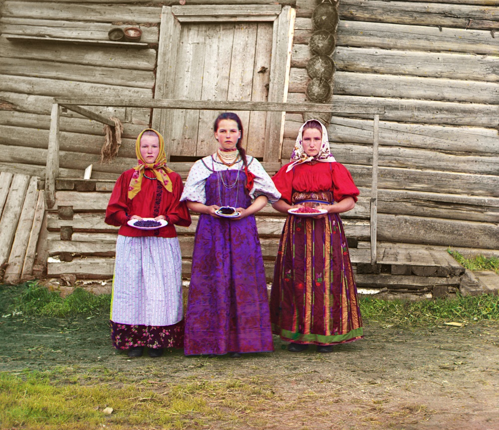
Many of the pictured we colorize looks over-saturated with blue and red. As illustrated in the following image (produced by our colorization algorithm our link), while the color for the dress looks rather vivid, the soil and the wood looks definitely unrealistic. I chose this image as the remapping baseline since it has many hues and colors and is representative of many of issues the original color space has.

Here is a professionally-retouched image I found online and our goal is to find the color remapping so that the baseline is more aligned to this target in terms of color.
Implementation
This is a histogram matching problem. Once we find a matching for the baseline and the target image, we can apply the mapping to all other images. The way I find the matching is simple:
- Find the cumulative histogram for both baseline and target.
- Find the piecewise linear interpolant f between the two CDFs.
- Find the discrete data points valued at x on the interpolated function f. x ranges from 0 to 255, and f(x) is the remapping.
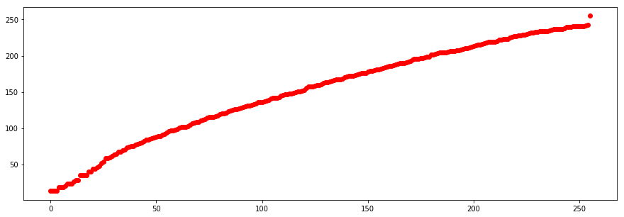
Here are the mappings I got for blue, green, and red. As expected, the mapping compensates the green channel by aggressively pushing up its middling intensity.
Results
Applying the remapping makes the color more natural but the image as a whole looks too bright and over-exposed. Thus, the next step is to implement a color balancing post-process.

(BELLS & WHISTLES) Color Balancing

I implemented a simple color balancing which clips the color intensity at [2.5, 97.5] percentile in each channel. Then, I stretched and normalized the channel histogram so that it distributes across the whole [0, 255] range. This balancing algorithm is added on top of color space remapping.