CS194-26 Project 1: Colorizing the Prokudin-Gorskii Collection
Hersh Sanghvi | cs194-26-add
The purpose of this project is to produce colorized versions of the photographs taken of the Russian Empire by Sergey Prokudin-Gorskii. Since he took these photographs when there wasn't a method to produce or display colored photos, he developed an interesting solution: for each subject, he fixed a red, green, and blue filter to the front of his camera and took shots with each of these filters. The LoC purchased his original glass plate negatives and made them available online. This project aims to produce colorized versions from the R, G, and B frames by aligning them and then stacking them into the RGB format.
Naive Alignment
For smaller (more compressed) images, the intuitive solution is to simply manually align the images by testing each possible vertical and horizontal shift of the frames. This works fairly well when the search space is small. Using the blue frame as reference, I aligned the green and red frames to it.
I found that the best metric for similarity was a de-meaned, normalized cross correlation. So, prior to computing the NCC, I crop out the borders, (using a simple heuristic that the borders are less than 10% of the image), subtract the mean from each of the images, and take the absolute value of the result to prevent overflow, and cast the result back to a uint8 (0 - 255). This works well at eliminating brightness differences between frames and emphasizing the edges. In fact, the de-meaned NCC in all cases performs as well as a Sobel (edge) based alignment. Here are the results for the small images (each finished running in 3-4 seconds), with offsets listed in (row, column) format.
Alignment Using Image Pyramids
For larger (on the order of 4000x4000) images, such as the .tif example images, the naive approach
would be too computationally intensive. Therefore, I use downsampling
to speed up the algorithm. I halve the number of pixels in the image (taking every other pixel)
per iteration, and then interpolate to avoid aliasing (using skimage.transform.resize).
This allows me to vastly speed up the search, since I can do a coarse alignment
at the lowest downsampled level (taking every 32nd pixel, or 2^5), and then I know that for
the next level up, the maximum possible adjustment is 2 pixels in the upper level.
At each level, I call the same naive alignment algorithm as before, passing in a maximum possible x and y displacement of
2 pixels. This leads to computation times on the order of 12 seconds for all the large images. The results are shown below.
For these, I used an initial displacement of 200 pixels, which was sufficient in all cases.
Bells & Whistles
Contrast Adjustment
Contrast adjustment refers to the spread of the pixel values in the image. A high contrast
means that the darkest pixels are concentrated around 0 while the brightest pixels are
concentrated around 255. I realized that if you approximate the pixel distribution as
Gaussian, then contrast refers to the variance of that distribution. To increase the variance of
a Gaussian distribution, you simply have to multiply it by a constant factor. My approach to
contrast adjustment was to multiply the image by a factor between 1.3 and 1.5, then subtract a
constant factor to bring the new mean back to the original mean. Results are shown at the end.
Icon, turkmen, and self-portrait look particularly good after this process.
Auto-Cropping
In lieu of more complicated methods for auto-cropping, my approach was to simply take the
mean of the rows and columns at the edges, until they approached non-extreme values. I check if the
mean of the row is less than 40 or greater than 230, and if it is, I consider that a border and crop it.
I do that until I encounter a row/column whose mean is greater than 40 and less than 230. This approach works
reasonably well for many of the images.
Sobel
In practice, a better way of doing alignment is based on edges. This is what the Sobel
edge detector does; it essentially transforms the image into its edges by passing it through
a bandpass filter. I found that doing this didn't yield any improved results over the
de-meaned NCC, though, so I didn't use it. However, I did find that it invariably reduced computation times,
from 12 seconds to 8-9 seconds. This is most likely because the image is sparser, so computing the cross
correlations becomes faster.
Results
Extra Images
HTML/CSS for organizing and displaying images taken from
w3schools.com
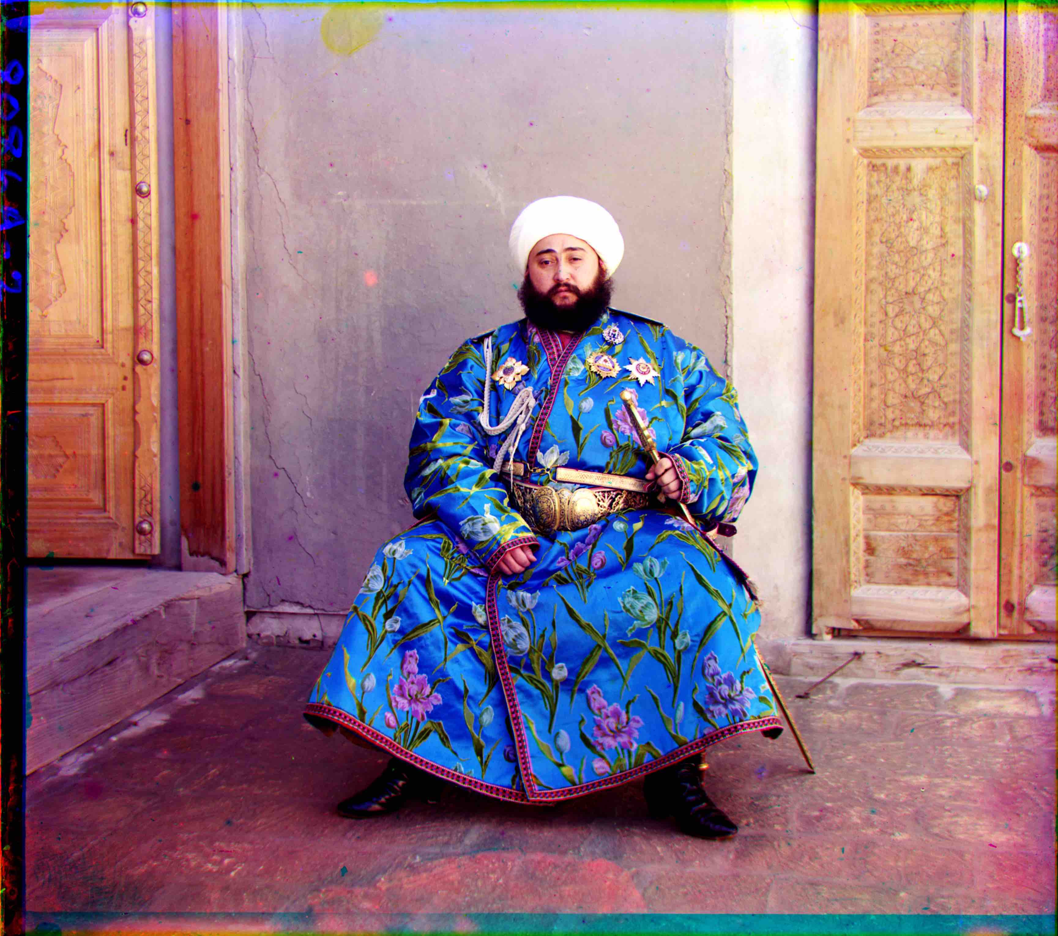
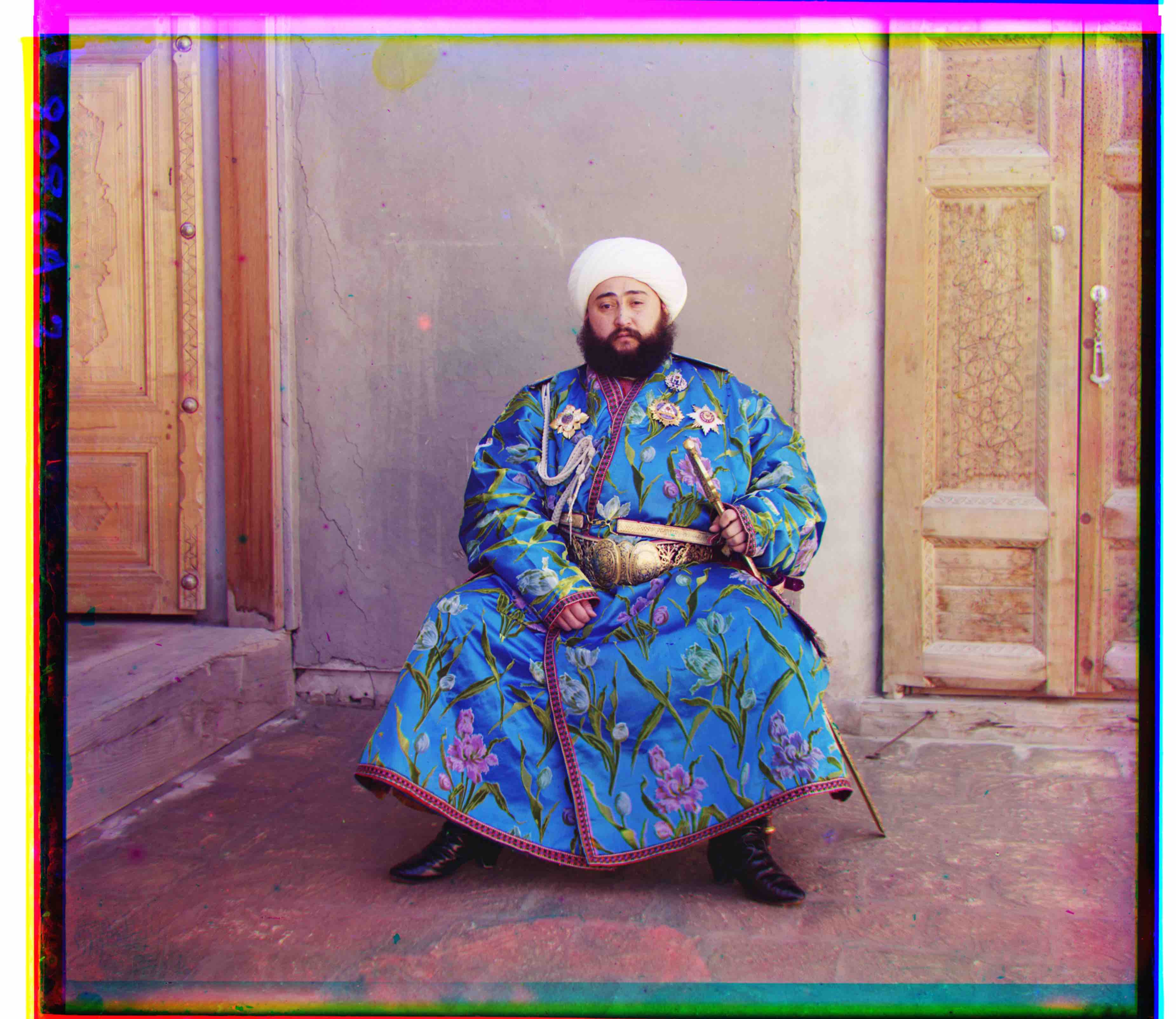 Emir: R(106, 41) G(49, 23)
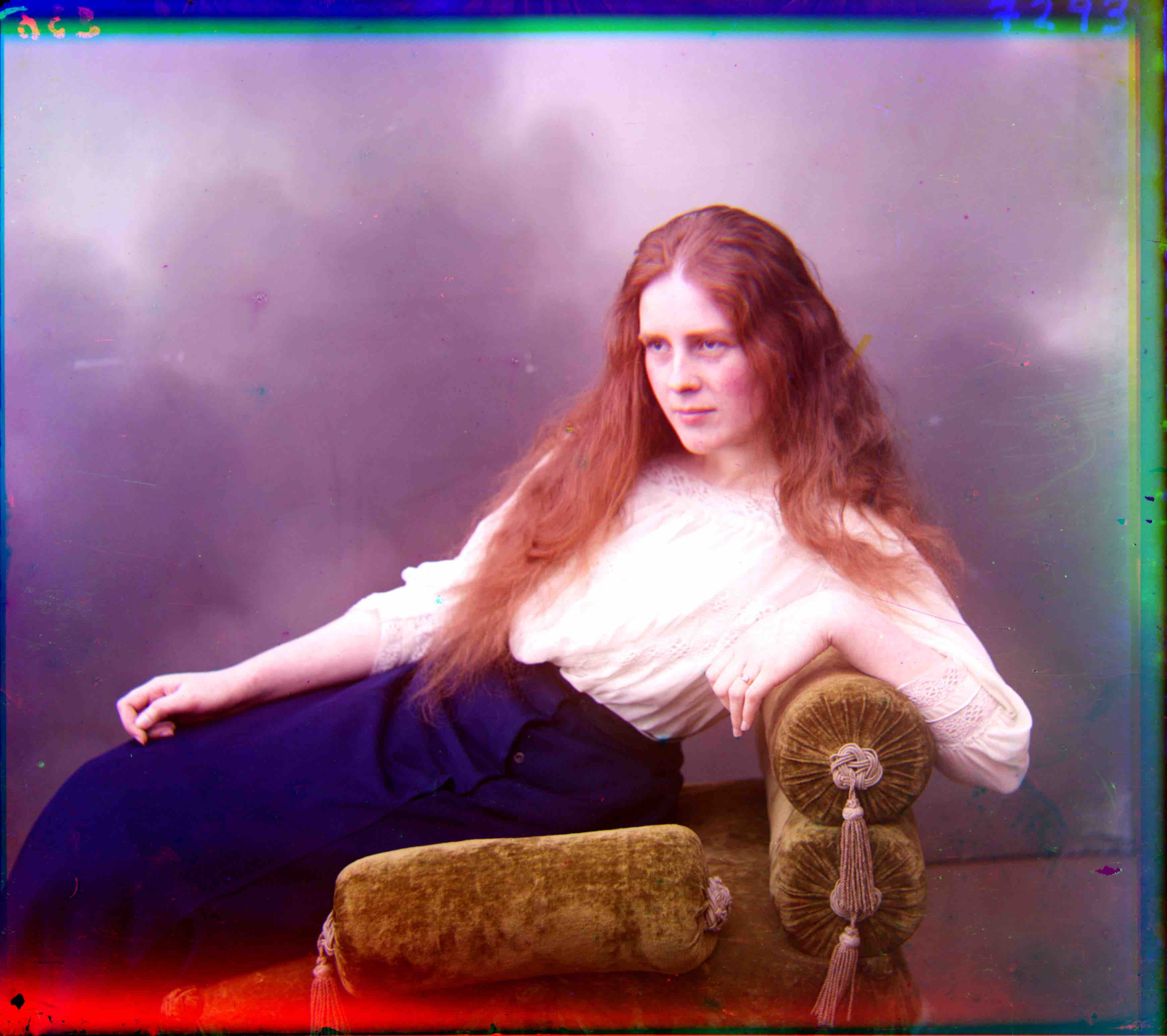
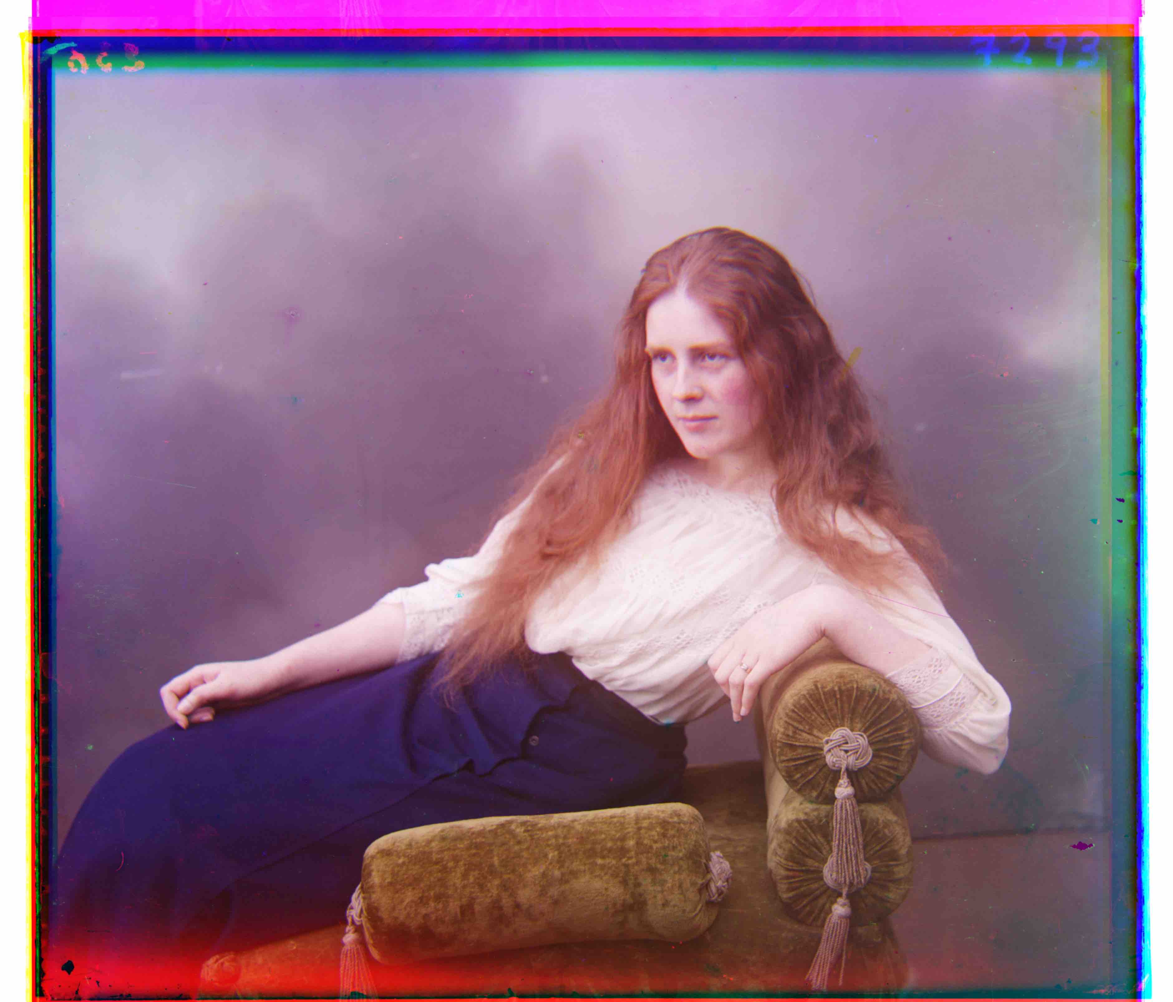 Lady: R(117, 11) G(54, 8)
![]() Icon: R(88, 23) G(40, 17)
Icon: R(88, 23) G(40, 17)
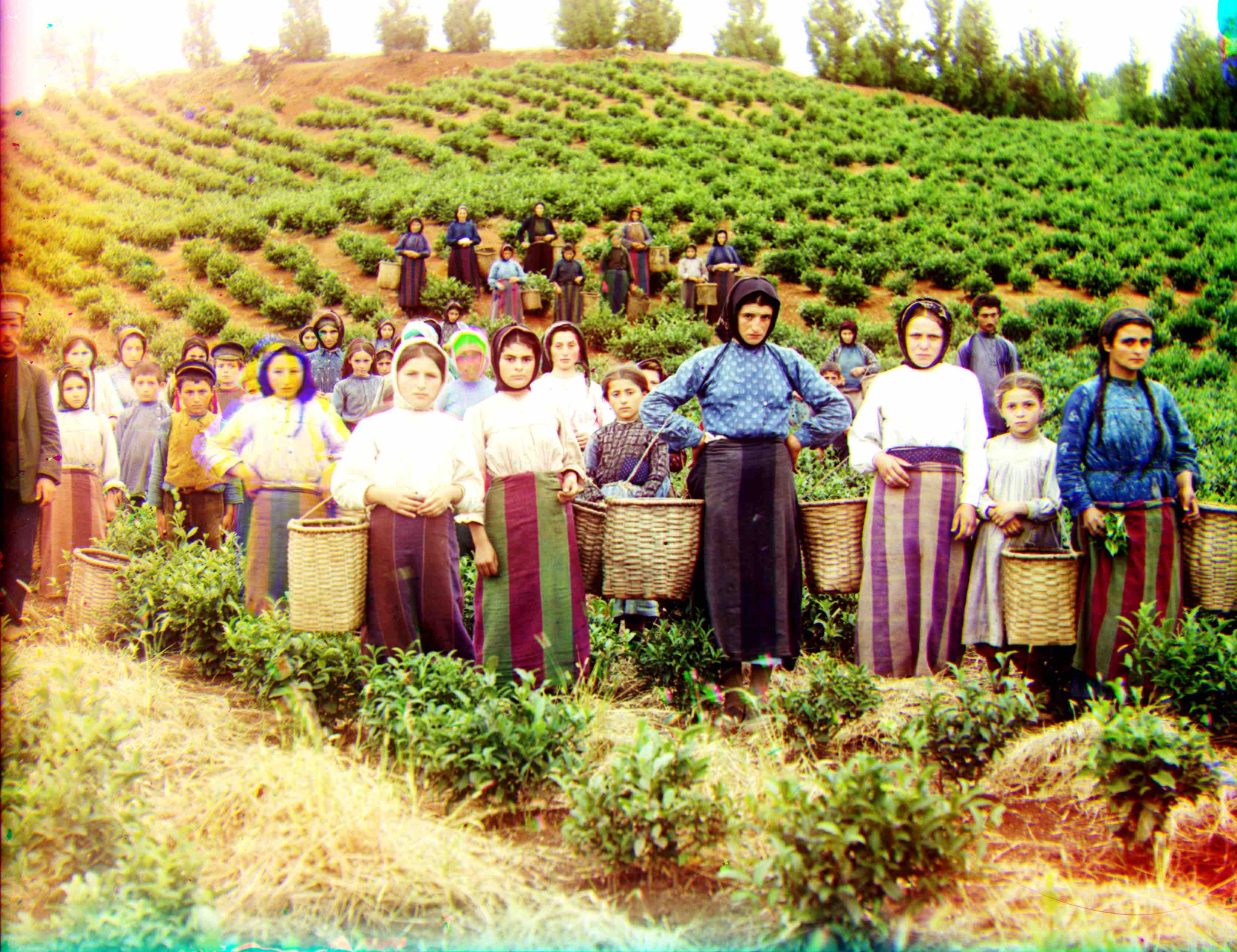
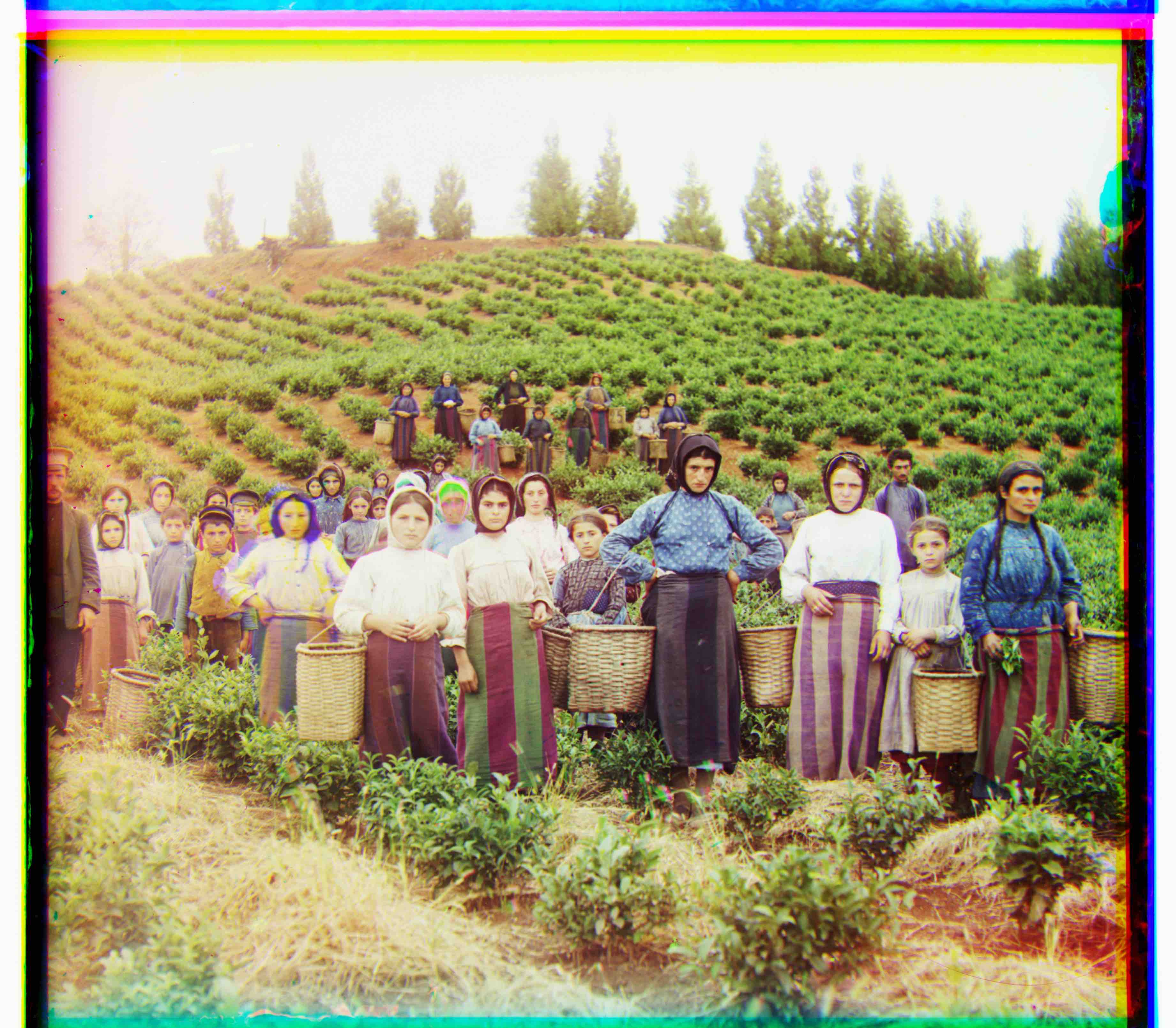 Harvesters: R(124, 14) G(60, 16)
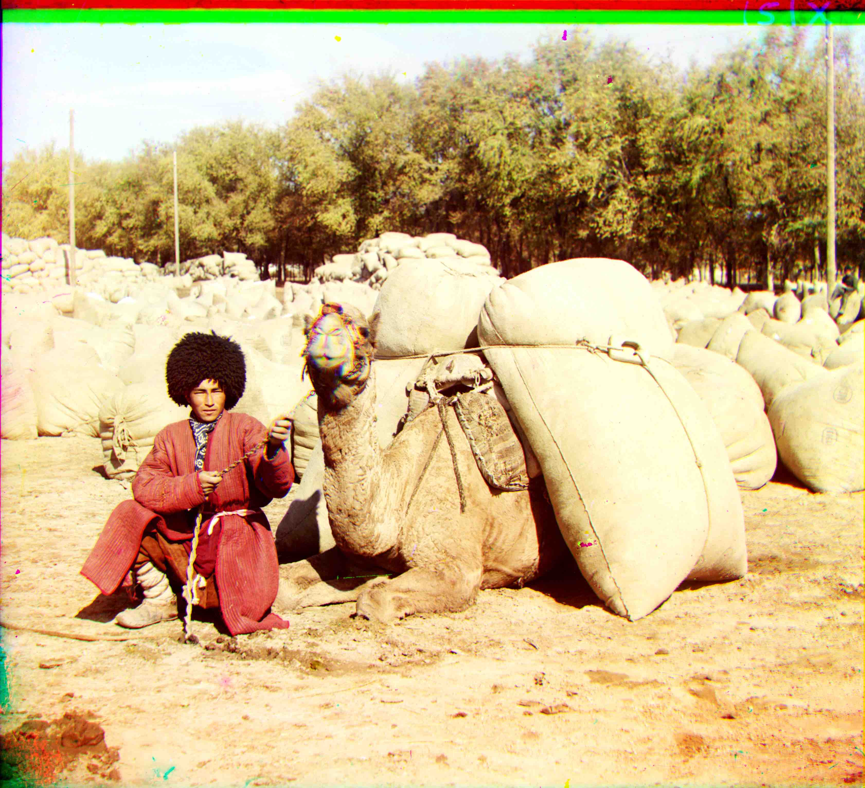
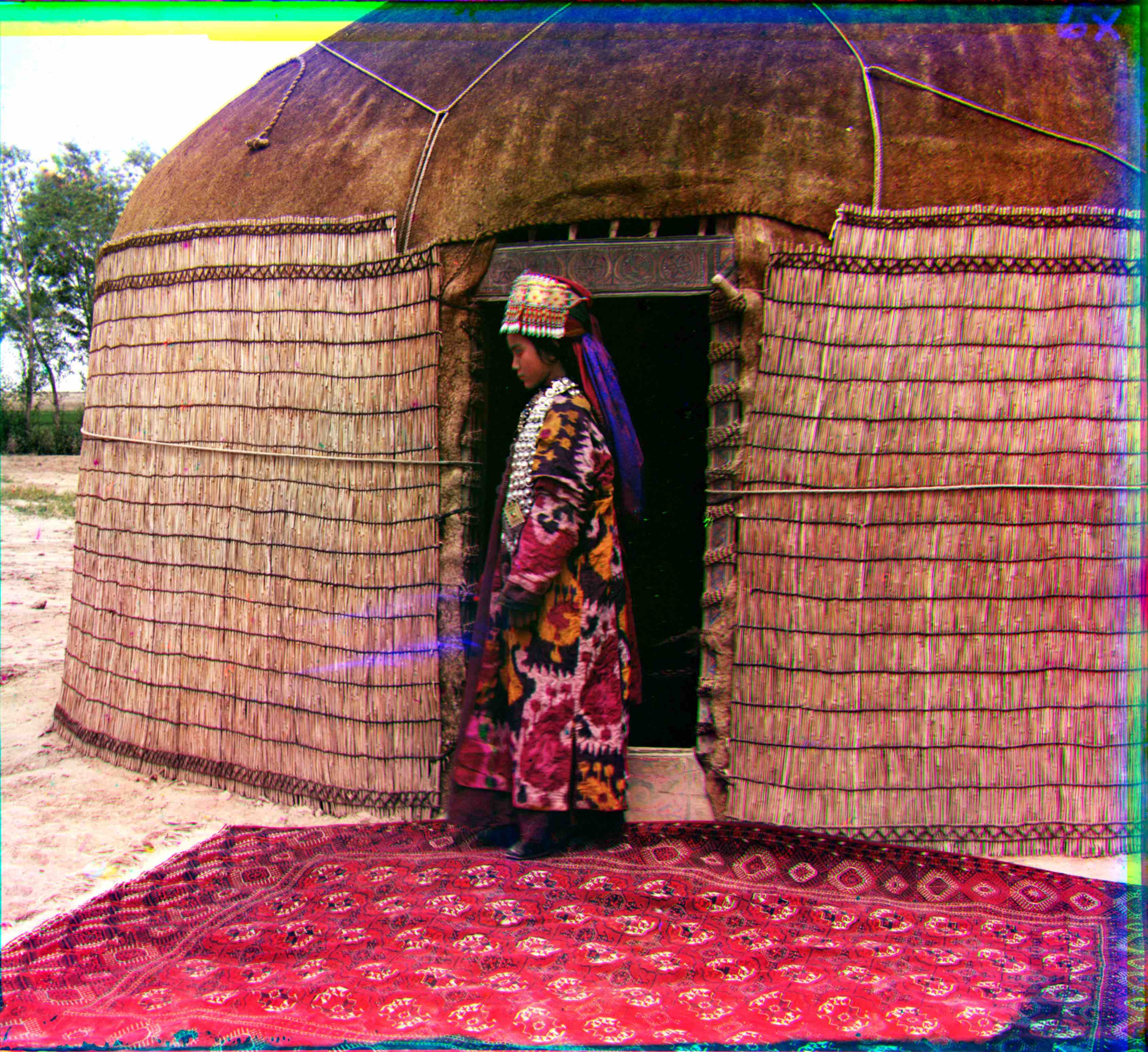
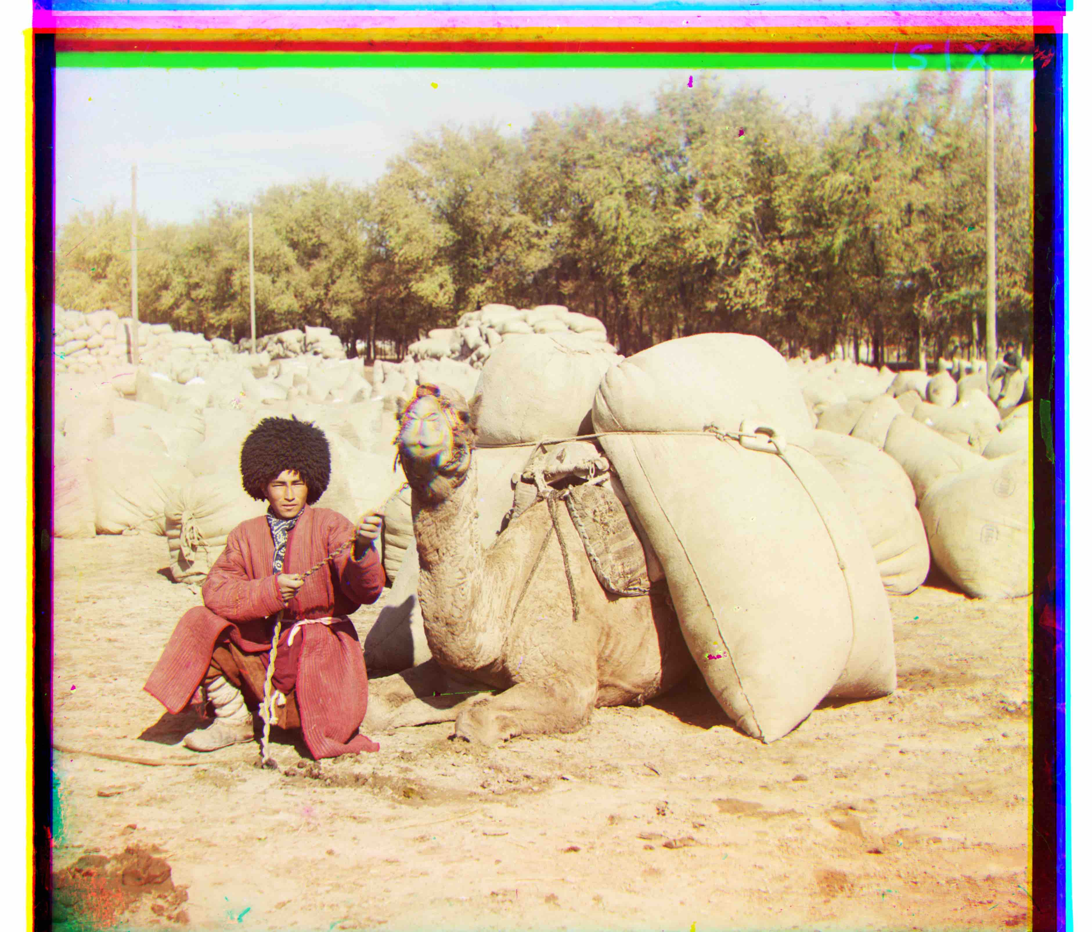 Turkmen: R(115, 29) G(55, 21)
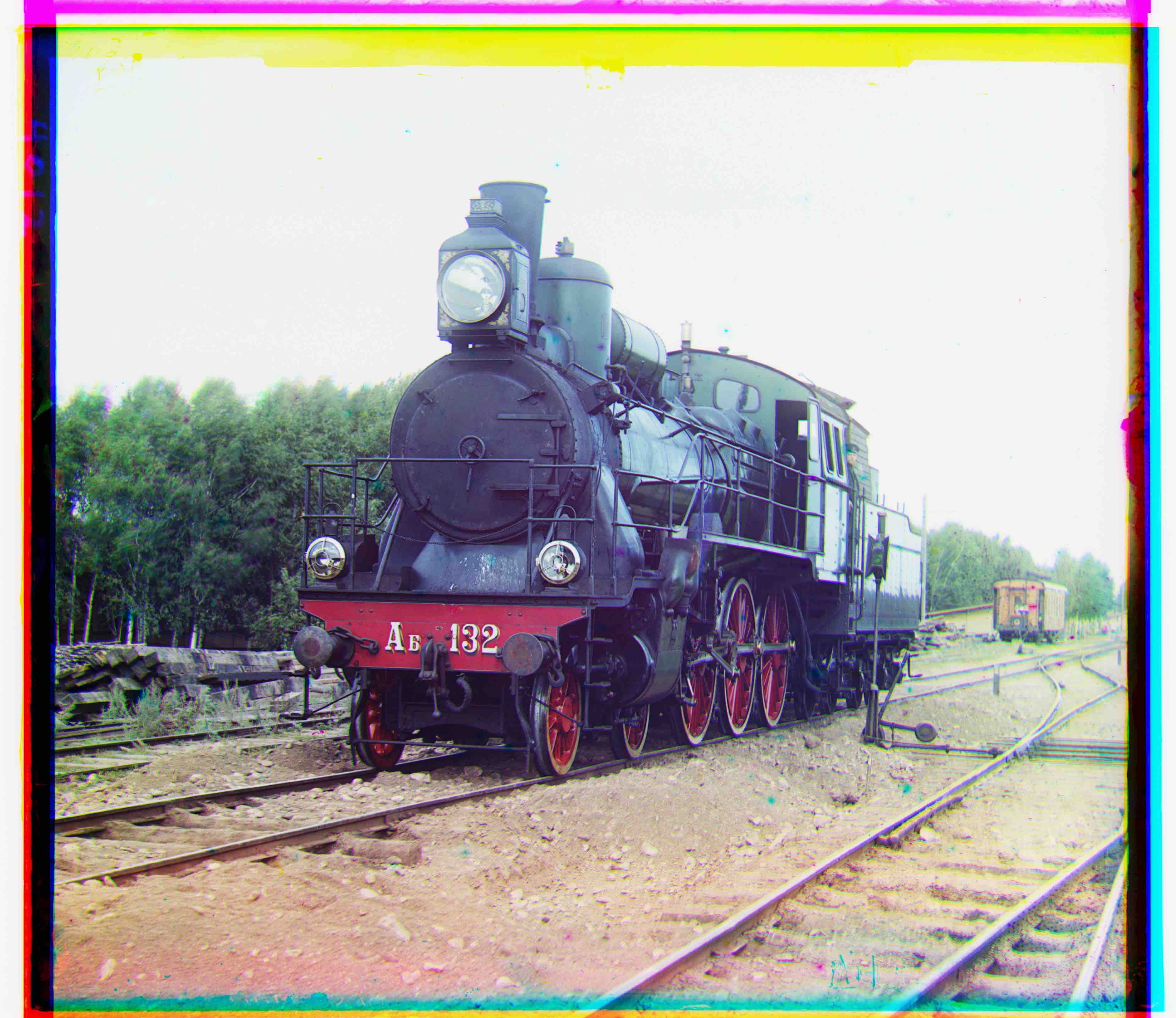 Train: R(86, 31) G(41, 5)
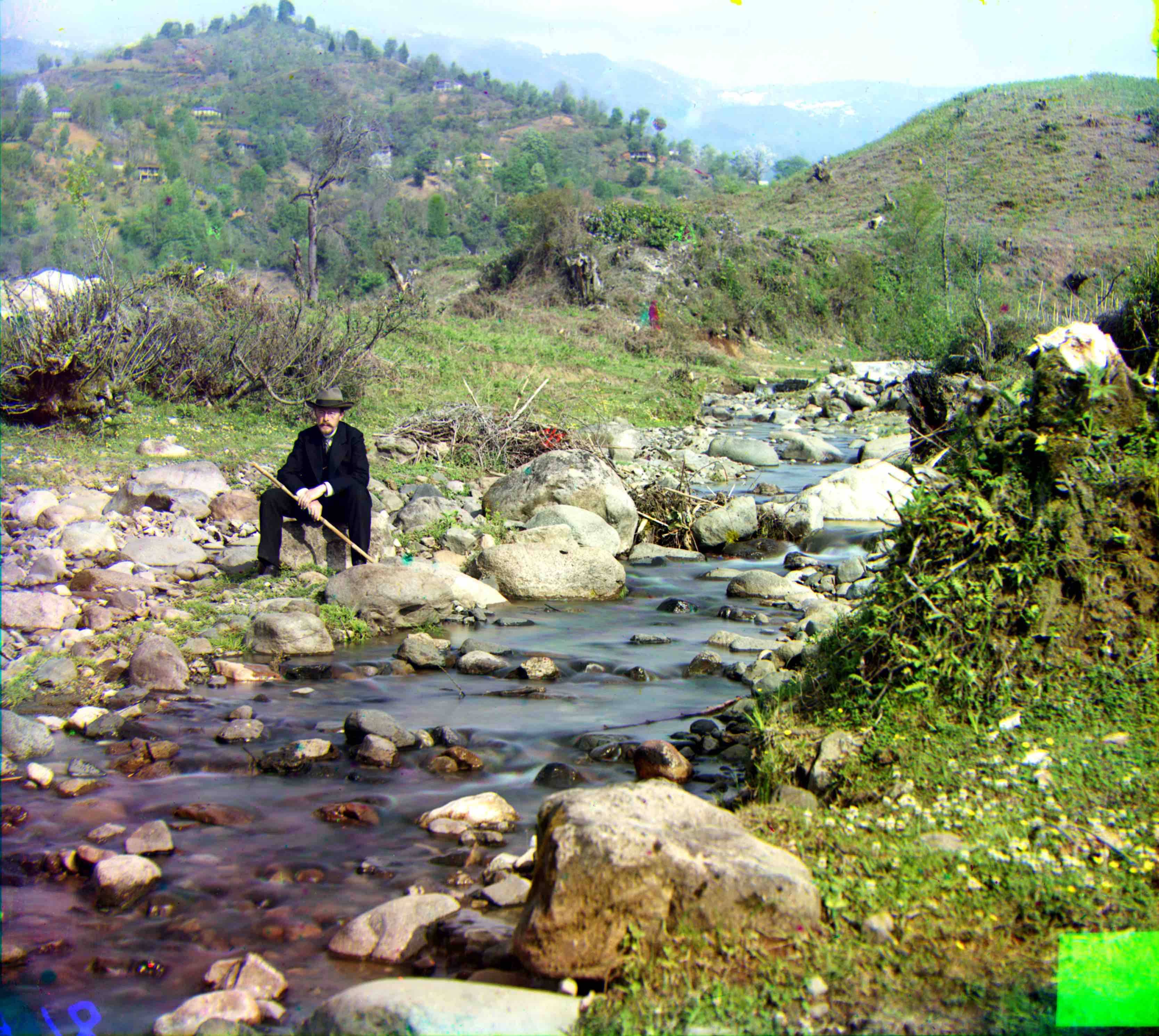
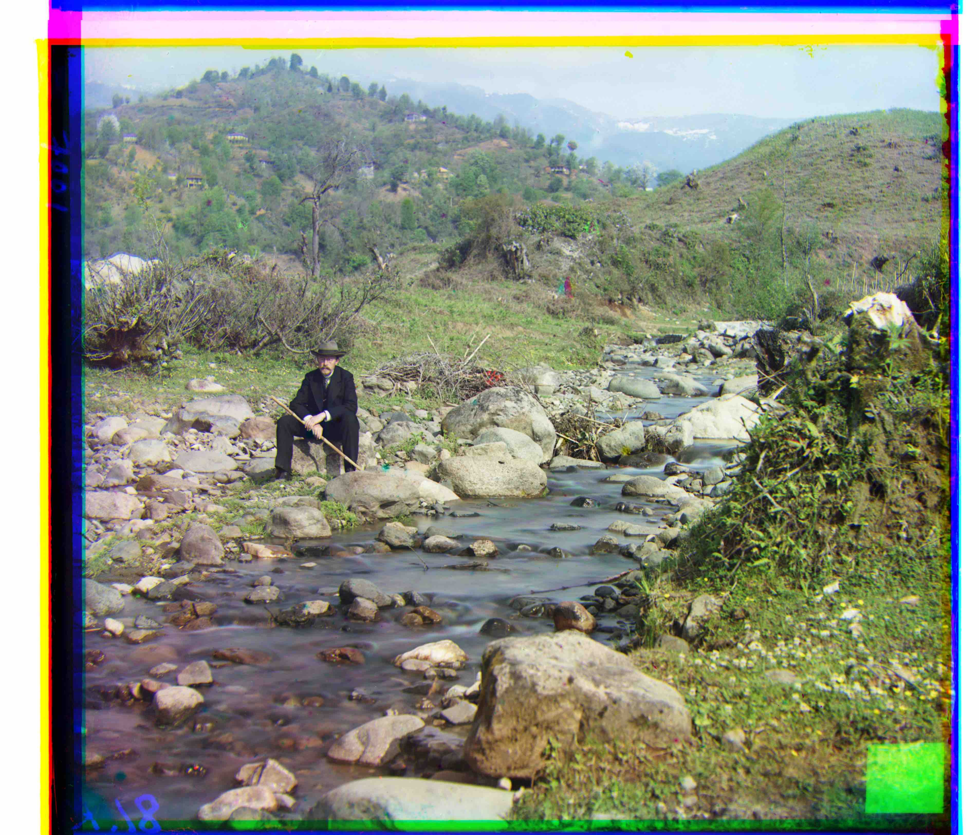 Self Portrait: R(175, 37) G(78, 29)
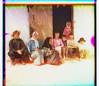
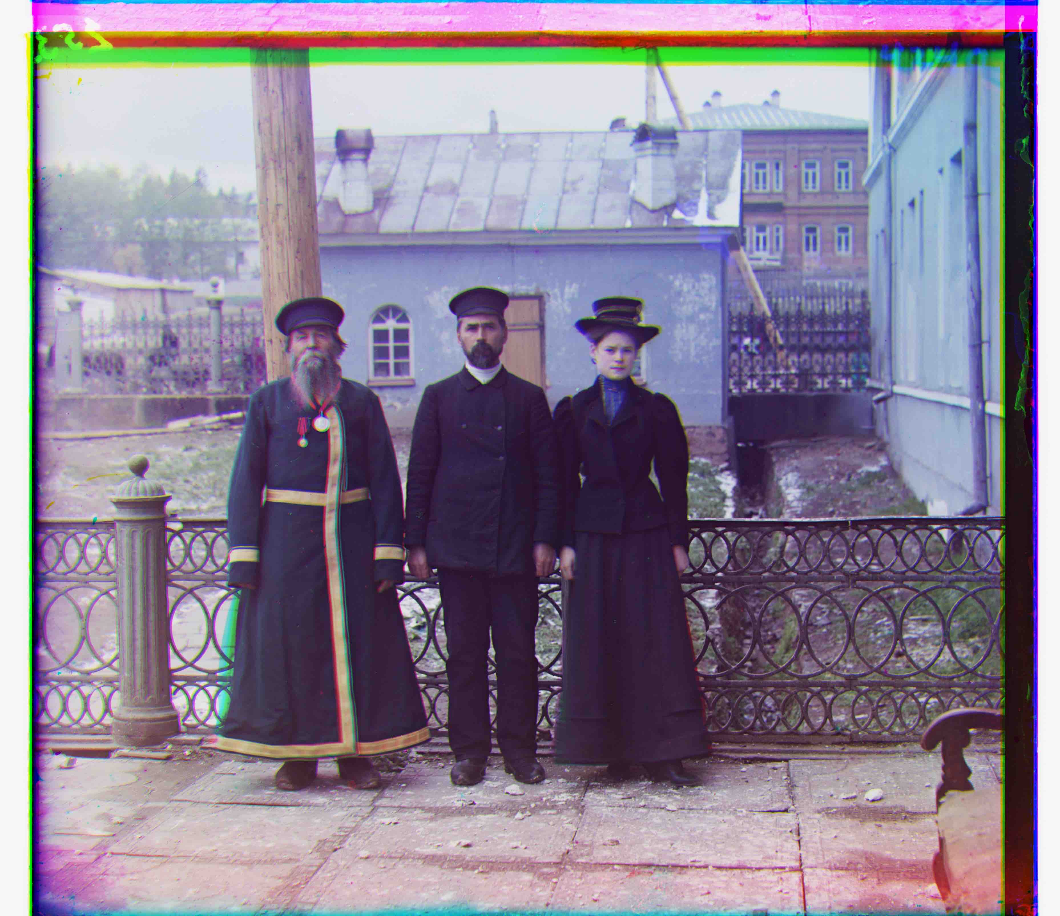 Three Generations: R(112, 10) G(54, 15)
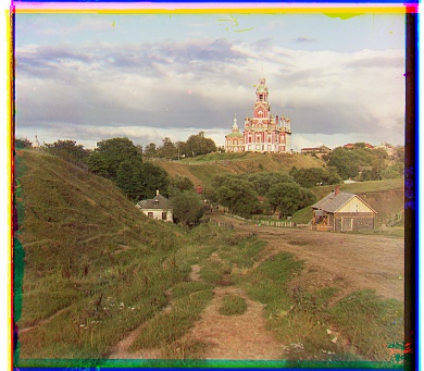
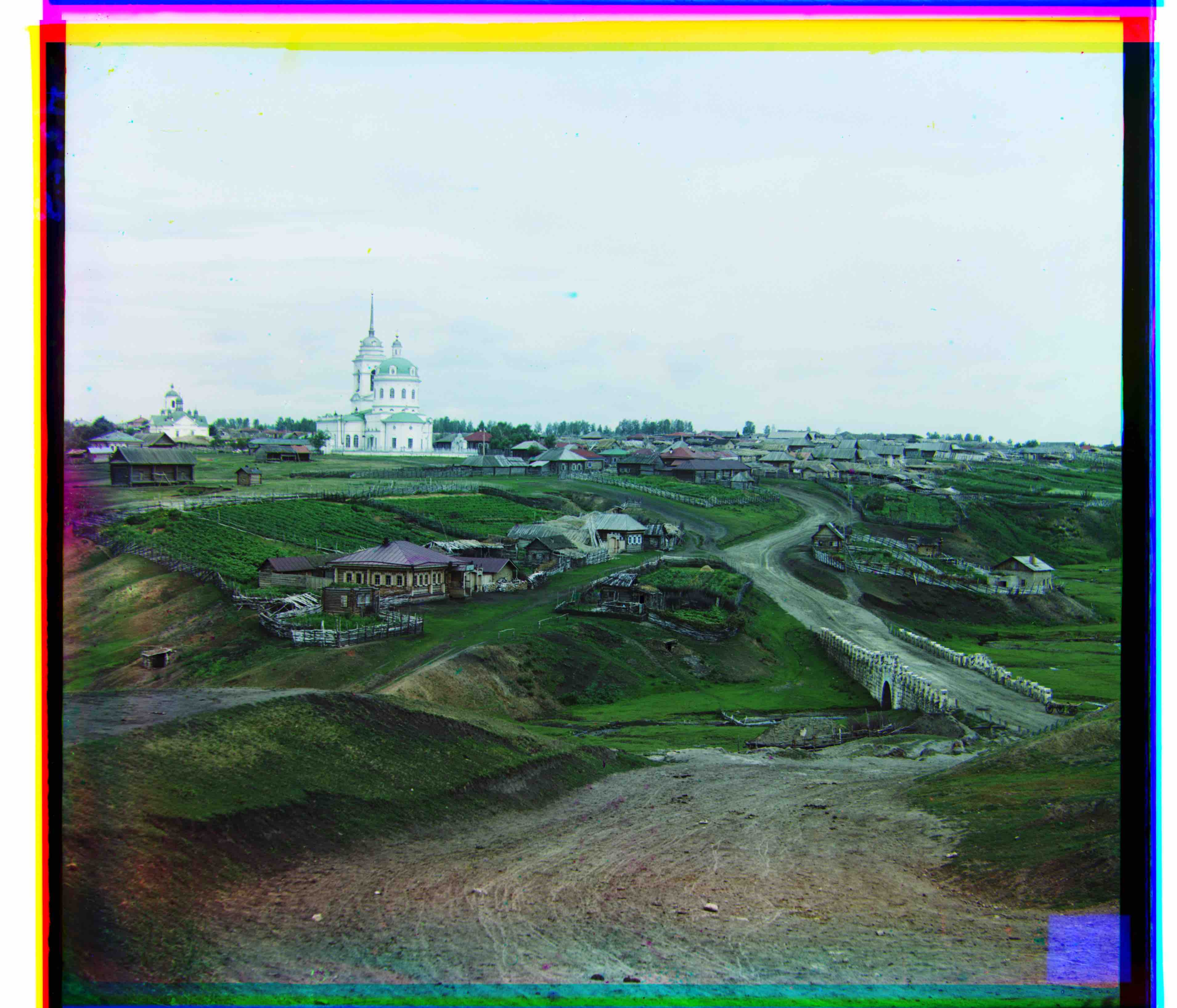 Village: R(137, 22) G(65, 12)
![]()

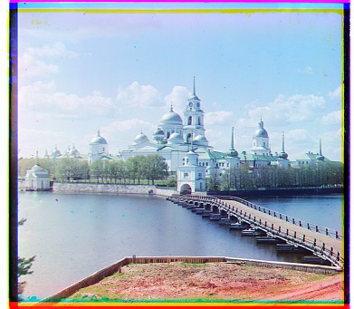
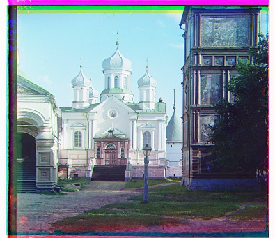
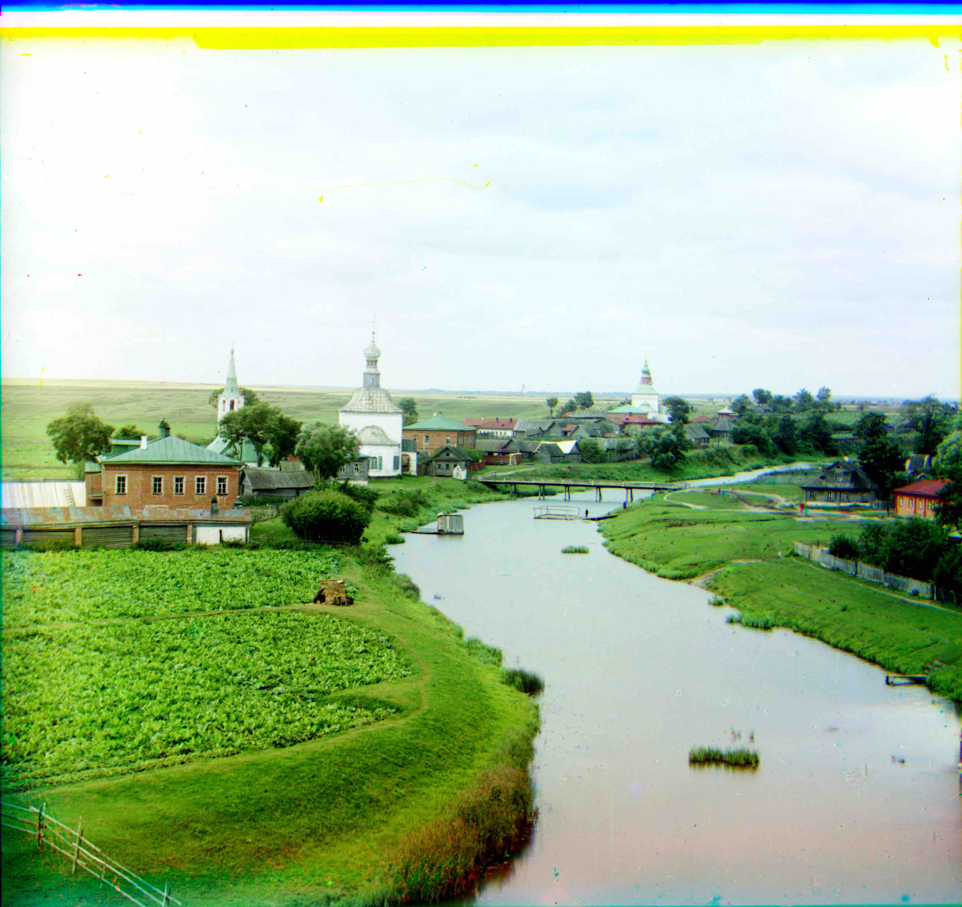 Suzdal: R(118, 3) G(55,8)
 Woman: R(68, 51) G(23, 36)
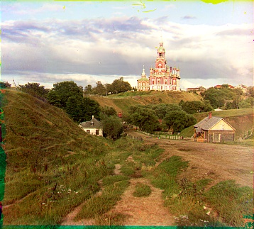
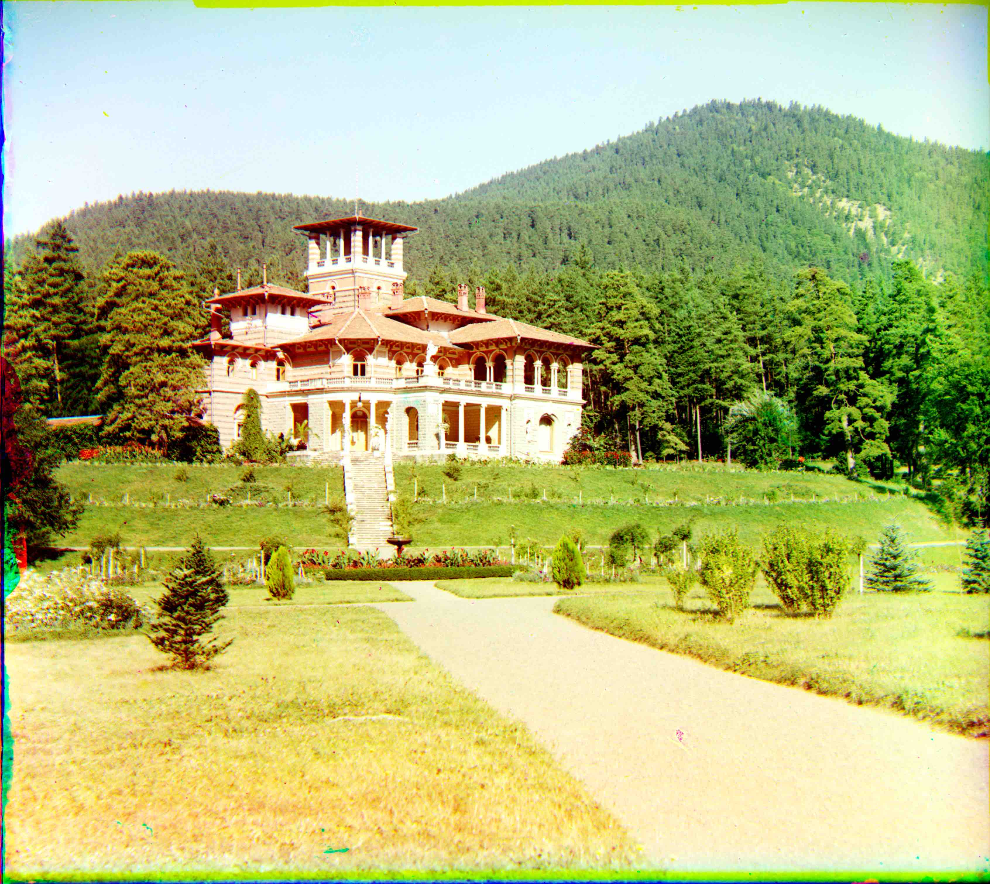 Likanskii: R(137, 7) G(59, 5)
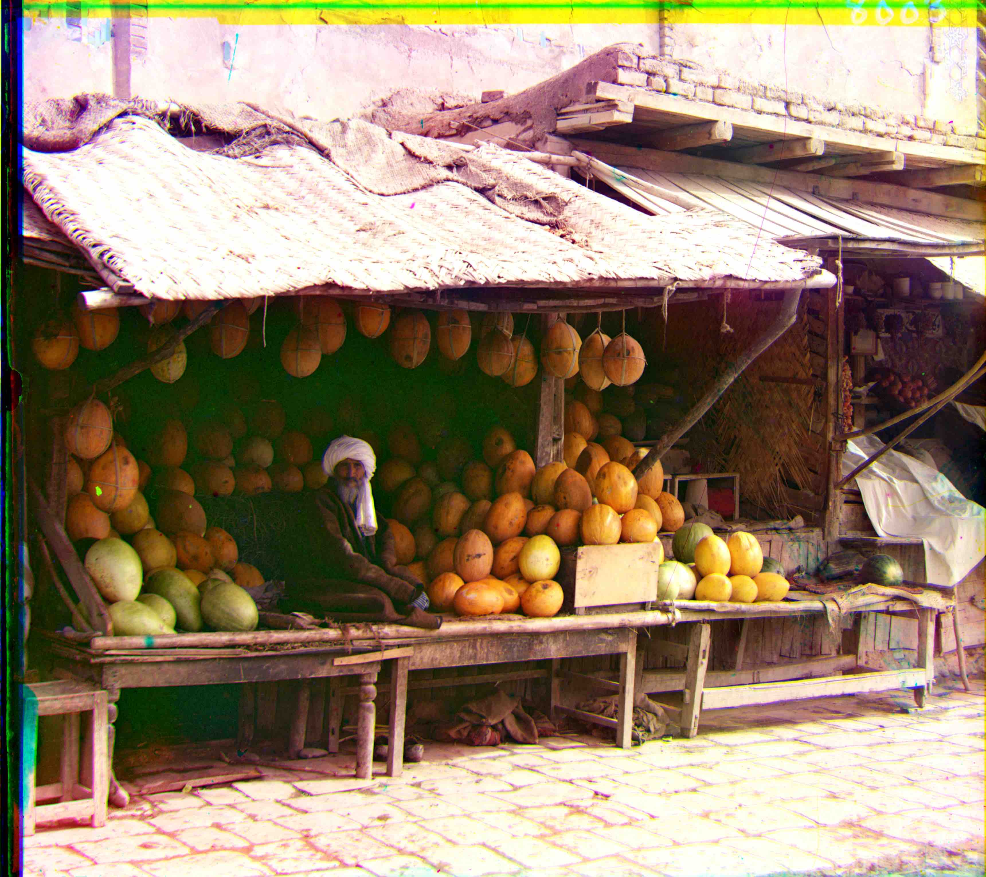 Melon Vendor: R(178, 13) G(81, 10)