Red Channel
Green Channel
Blue Channel
Images of the Russian Empire:
Colorizing the Prokudin-Gorskii photo collection
COMPSCI 194-26 // Project 1 // Fall 2018
By Naomi Jung // cs194-26-ads
The goal of this project was to use image processing techniques to combine glass-plated grayscale images taken using red, green, and blue filters to produce a colorized image. When the three plates are aligned on top of each other, the three color channels combine to form the colorized RBG image. Thus, the challenge was to find the optimal vector displacement for each of the color channels in aligning the images on top of each other.
The input image was a vertical strip of the three channel-specific images stacked on top of each other, and I began by splitting them into three equal parts, as shown above. Because the images had varying borders, I decided to crop the images by 7% so that the border pixels would not be factored into the matching algorithm and calculations.
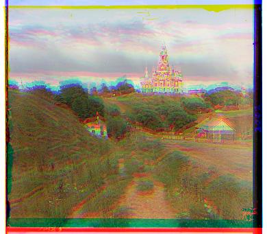
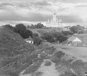
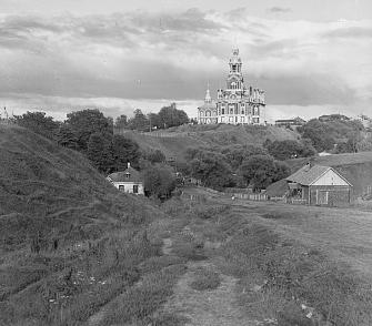
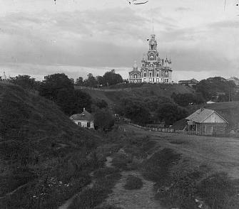
Before image processing, overlaying the three channels looked something like this. Here we can see that the channels are not correctly aligned, which is why we have the misaligned effect where we can somewhat see separate color channels on top of each other. Ideally, when we run the algorithm, we would align the first channel with the second channel, and we would repeat to align the first channel with the third channel, which would result in the image plates aligning to create a cohesive, blended, and colorized image.
In completing this project, I explored two main methods of image alignment: (1) naive processing that exhaustively computed a match score over a window of possible displacements and (2) an image pyramid algorithm that recursively scaled down the image by half in order to achieve a more optimal processing time.
As a note to the reader, the displacement vectors and processing times listed in the following sections for each image refer to the final vectors and times resulting from my final algorithm (the image pyramid algorithm) and not the more naive algorithms.
To begin, I implemented naive image matching. For images that were relatively small, namely the JPG files, I iteratively searched over a window of possible displacements of [-15, 15] to find the best displacement. I used the sum of squared differences (SSD) to compute the match score of each (x,y) displacement, and essentially chose the displacement vector (x,y) that produced the smallest SSD. I also experimented with using a match score involving the Normalized Cross-Correlation (NCC), which took the dot product of normalized vectors. However, with this metric, the runtime increased significantly, and I saw that there was not much difference in the resulting displacement vector and the result aligned image. Thus, I decided to use the SDD as my metric for finding the best displacement.
Ultimately, this method worked well for the smaller JPG images as shown below. Since we were only iterating through 225 different displacement vectors, the method was relatively fast. Furthermore, since the images were small, we could be confident that the displacement vectors were bounded by our hard-coded window of [-15,15].

We saw that the naive implementation was not going to work with the larger TIF files since they were likely to have optimal displacement vectors outside of our predetermined window, since the pixel-widths of these images were much larger. Iterating over such a large displacement window would be inefficient and take too long, so a more efficient solution was necessary.
Thus, I implemented an image pyramid algorithm that recursively searched for the optimal displacement vector going from a coarse, low resolution version of the image to the original fine, high resolution version of the image. While the image was greater than 100 pixels in height, I rescaled the image by 50% and searched for the displacement vector. Upon completing the recursive call for a coarse image, I doubled the values of the displacement vector to get the vector in the higher resolution image and searched for the optimal alignment over a small window near those values.
This algorithm proved to be much more efficient than the exhaustive search from the previous section because we were able to target our search for the optimal vector more effectively with each recursive step, instead of naively searching everything.
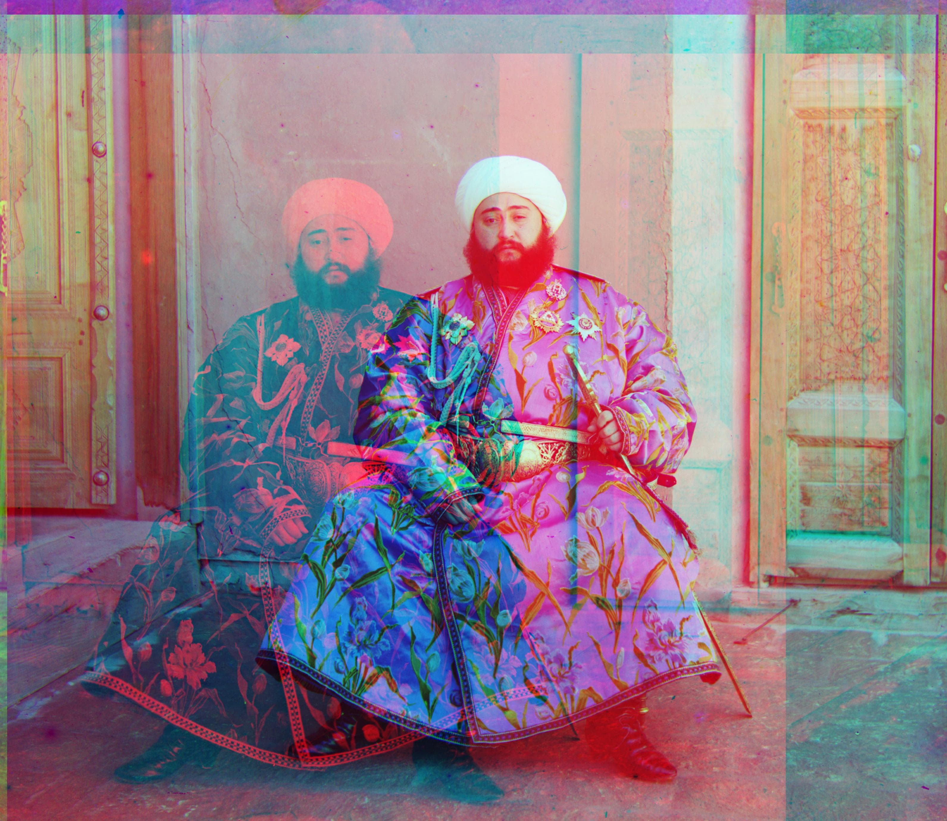
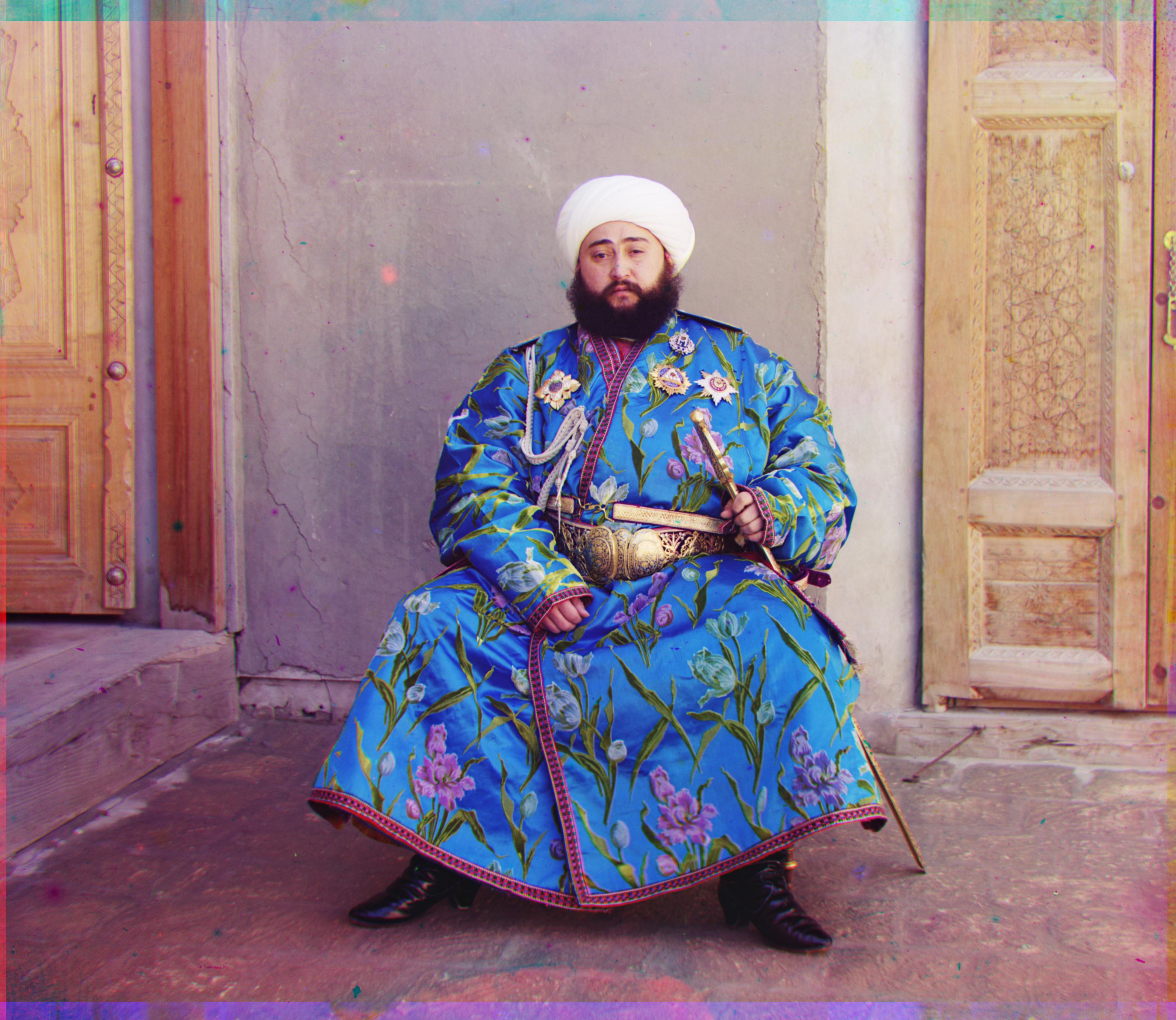
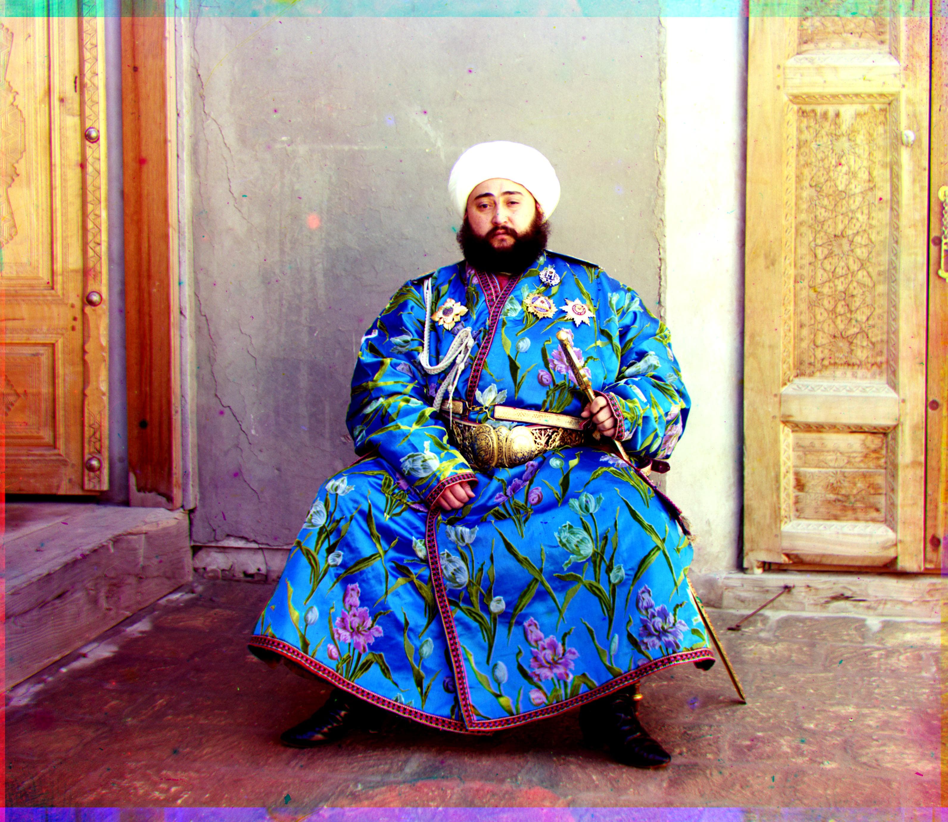
While working on this, I did come across a major alignment issue with emir.tif. When I ran the algorithm, I found that the red channel was way out of alignment. Initially, I had been using the blue channel as my alignment base, meaning that I had been aligning the red channel to the blue channel, and then the green channel to the blue channel. To solve this issue, I tried using the green channel as the alignment base instead, and aligned the blue channel to the green channel, and then the red channel to the green channel.
The switch to using the green channel as my base ended up fixing the issue and allowed all the channels to become aligned. This may have been the case because Emir's clothes are blue, and the high intensity of this channel along with the low intensity of the red channel prevented us from being able to match color channel intensities effectively. By using green as base, however, we were able to work around this and align the image.
Below are the colorized TIF images, with their runtimes and optimal displacement vectors.
To improve the image quality, I also looked into implementing auto contrasting for the images. Prior to alignment, for each color channel, I determined the 5th and 95th percentiles of the pixel values. Then, I used linear stretching to auto contrast the image. This meant that all pixel values less than the 5th percentile were set to 0, and all greater than the 95th percentile were set to 1. The middle 90% of values were stretched to span from 0 to 1, which increased the intensity of the pixels.
Below, I've provided a couple example "before" and "after" images showing the effects of my auto contrast algorithm.
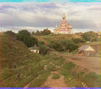
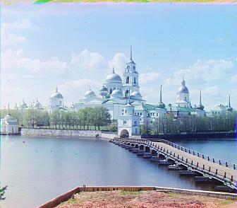
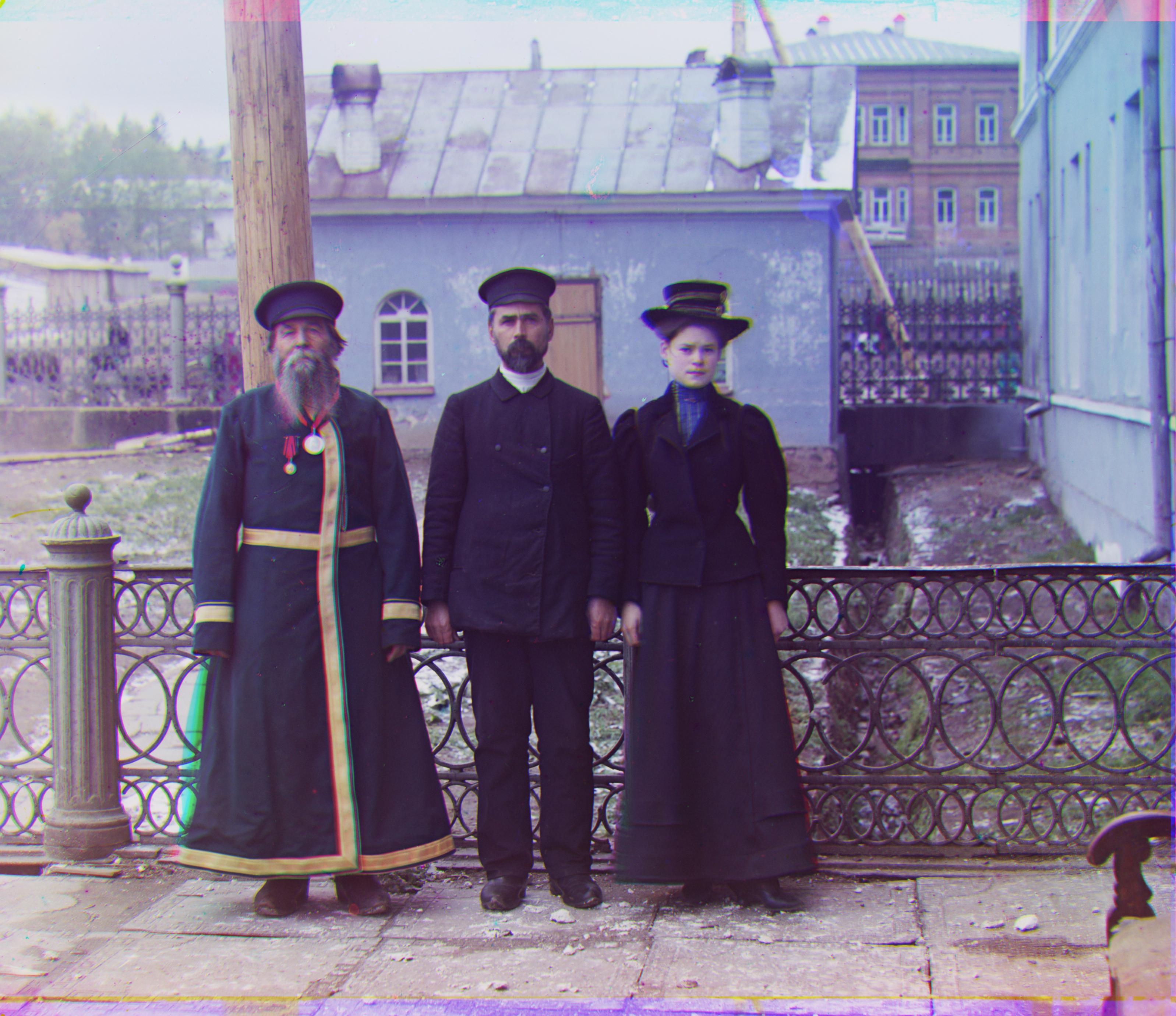
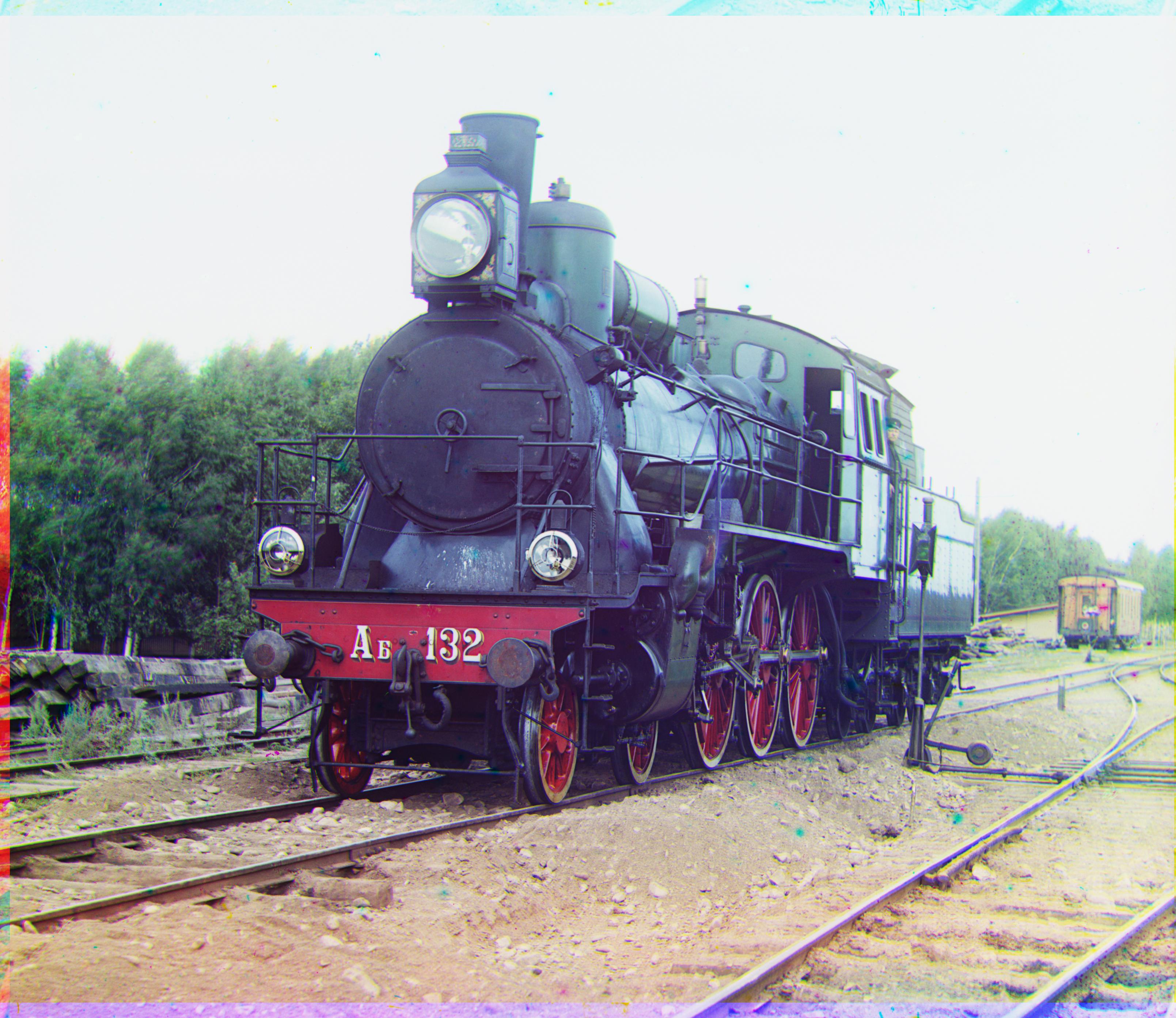
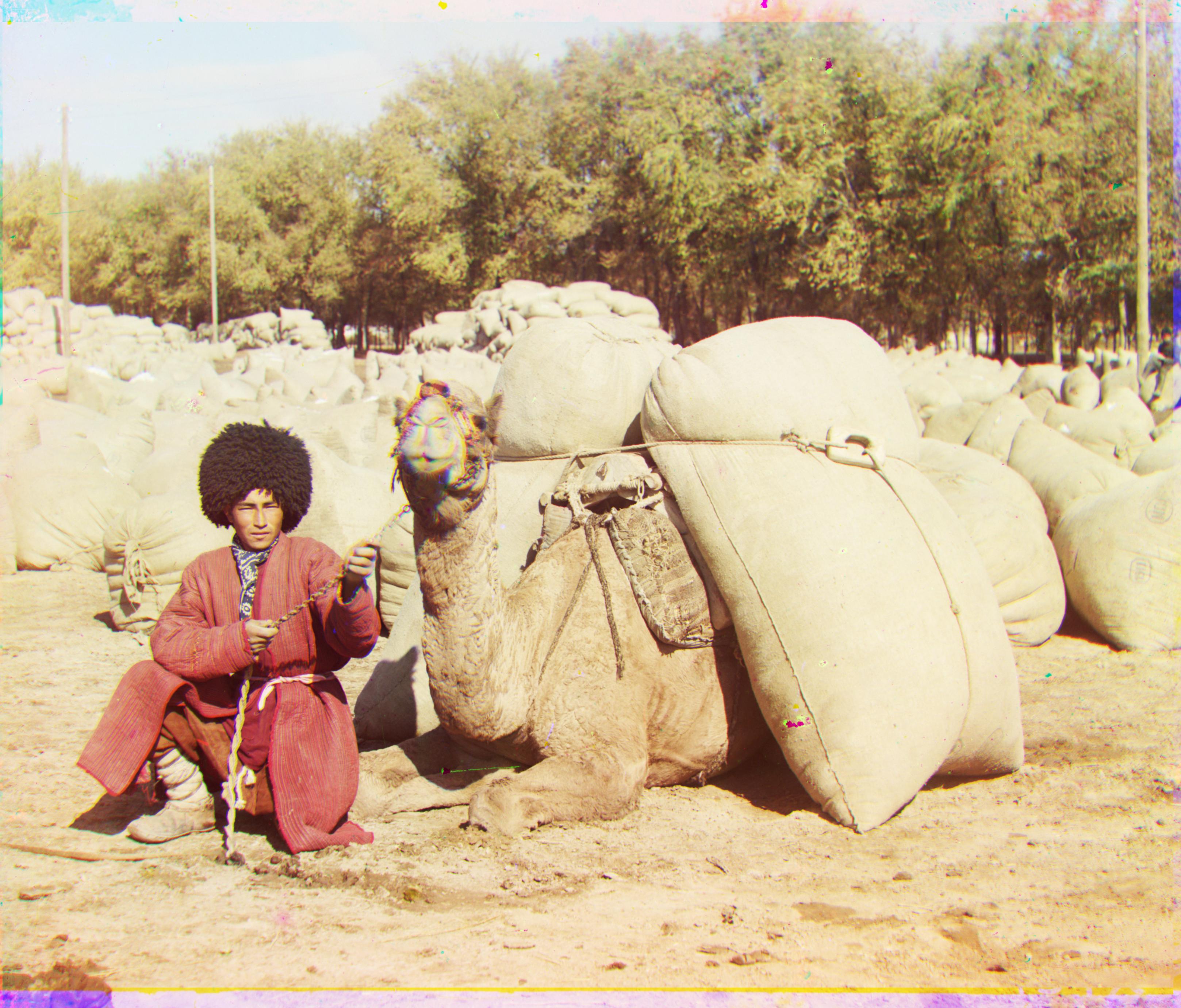
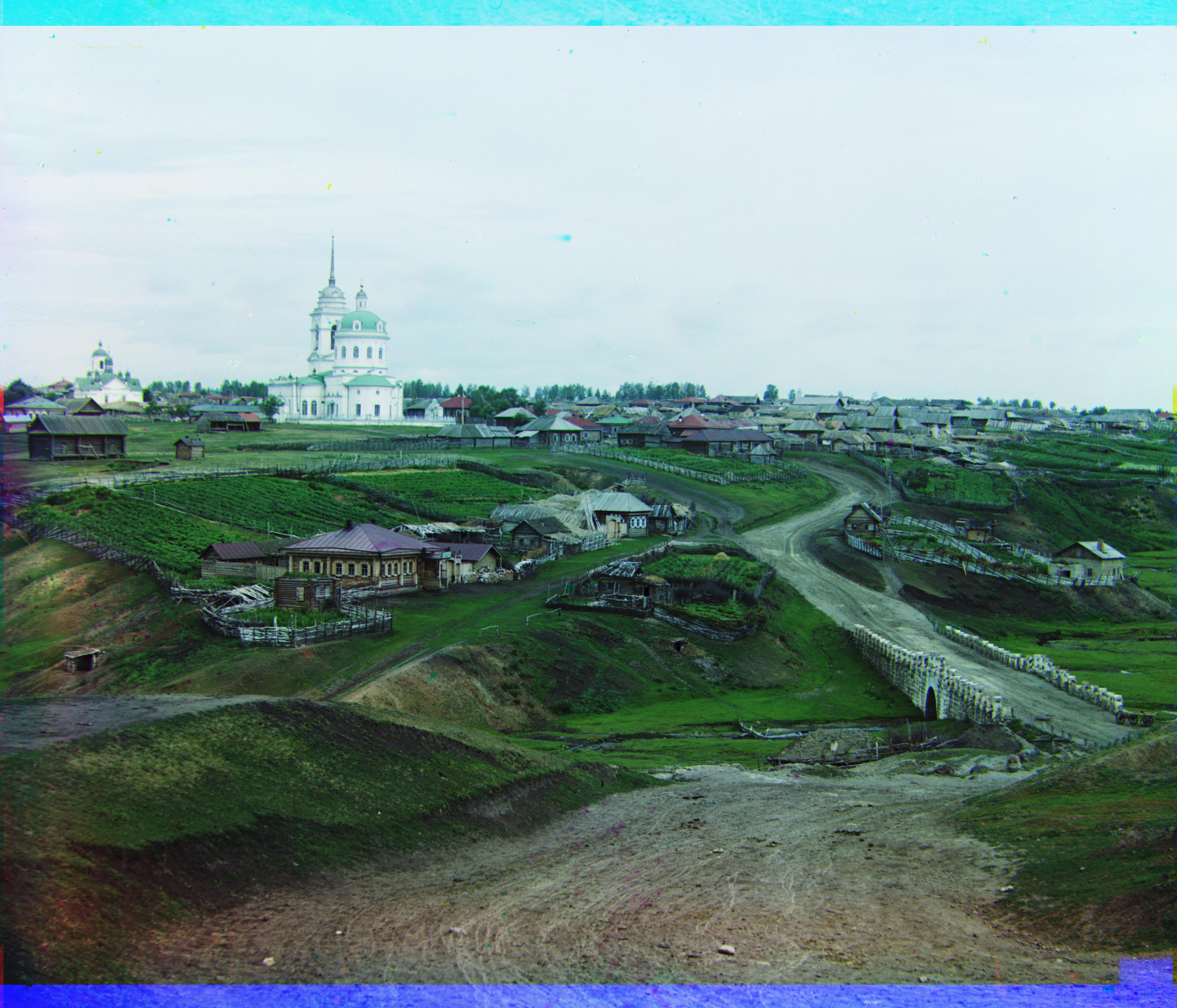
Here, I've listed all the example images, after running the full algorithm, which included the auto contrast.
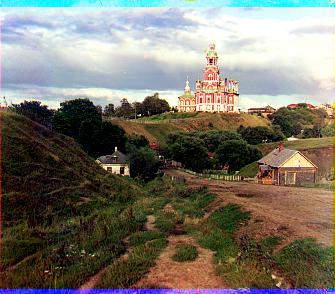
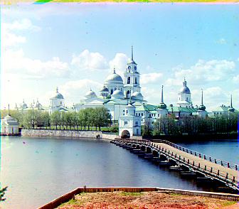
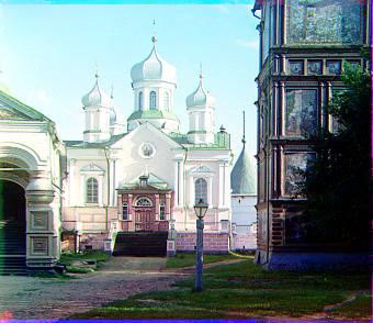
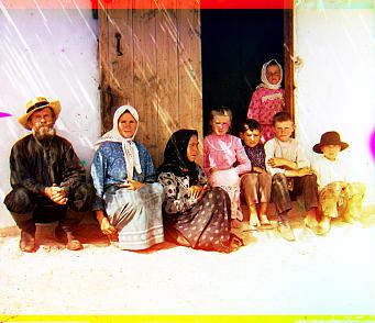
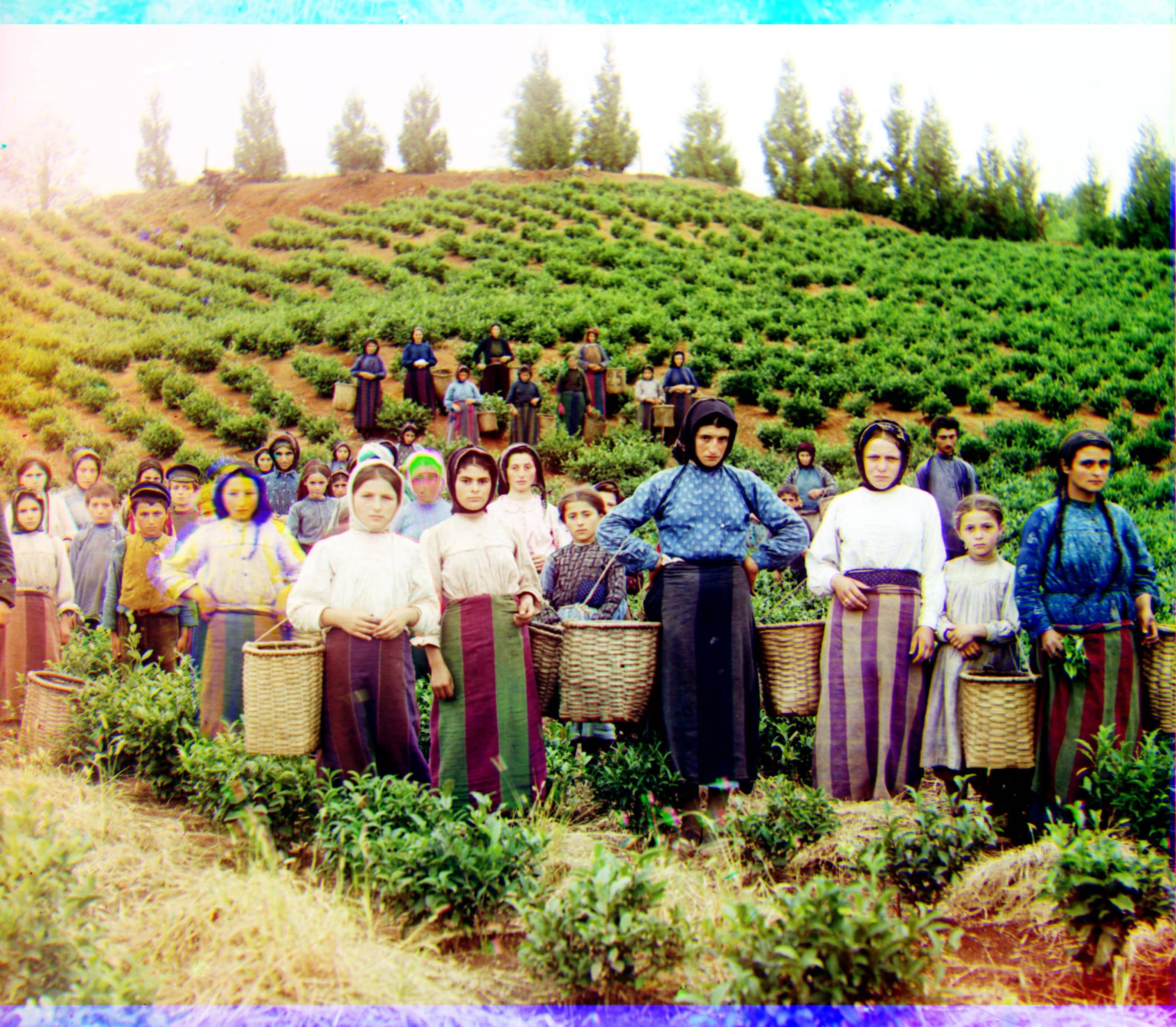
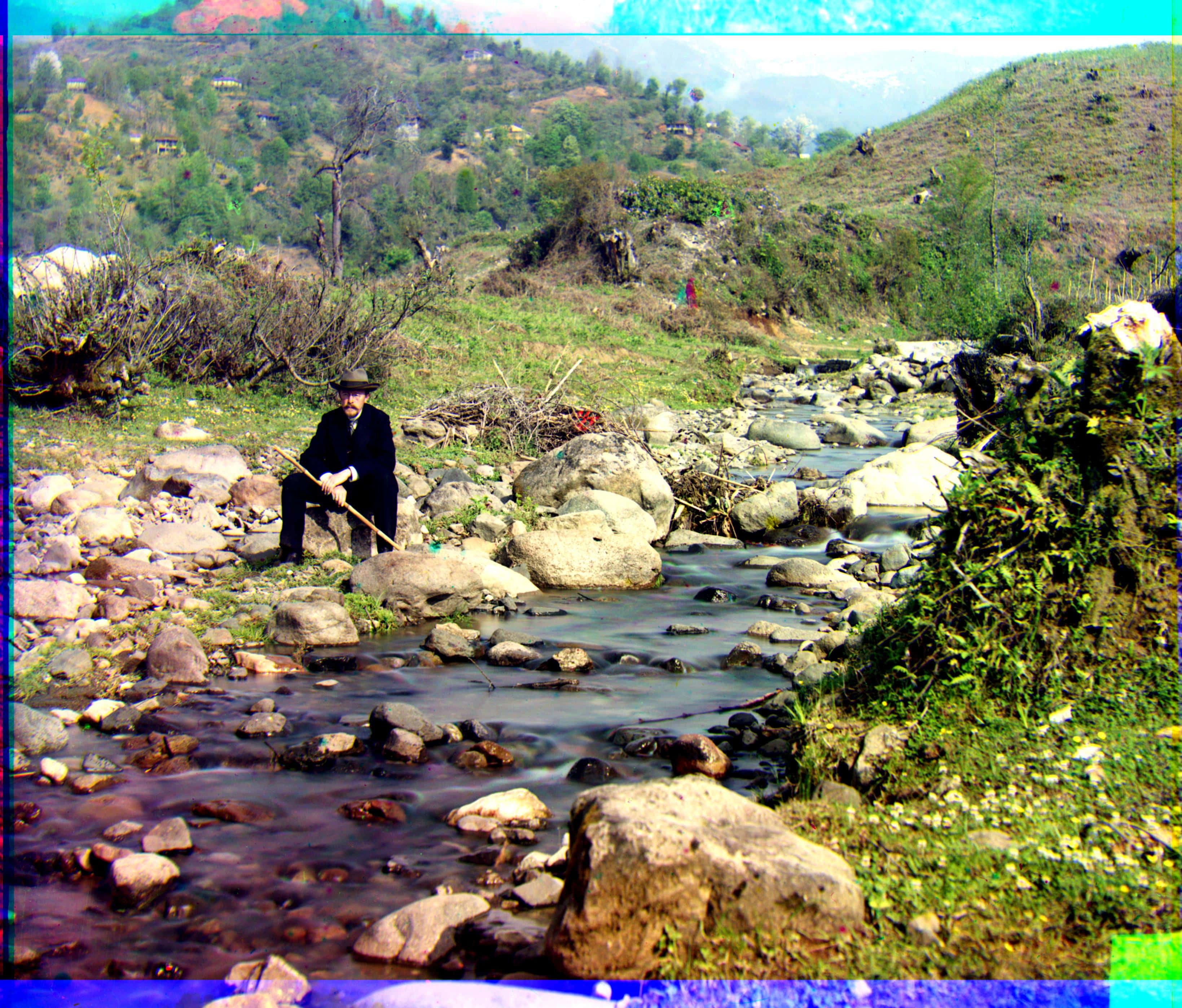
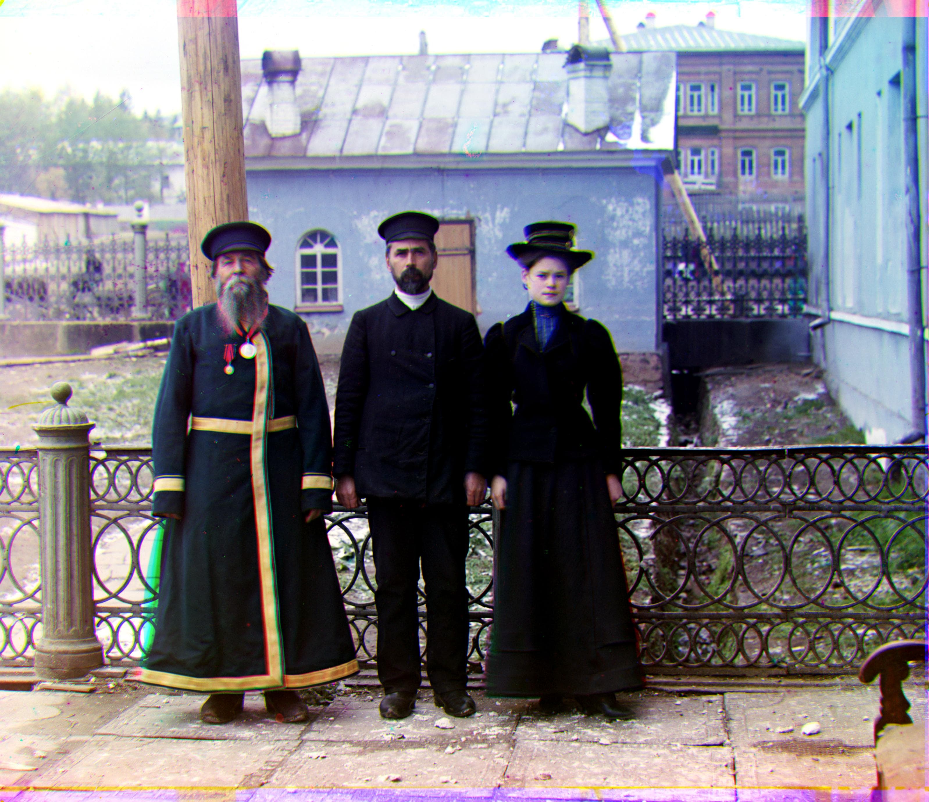
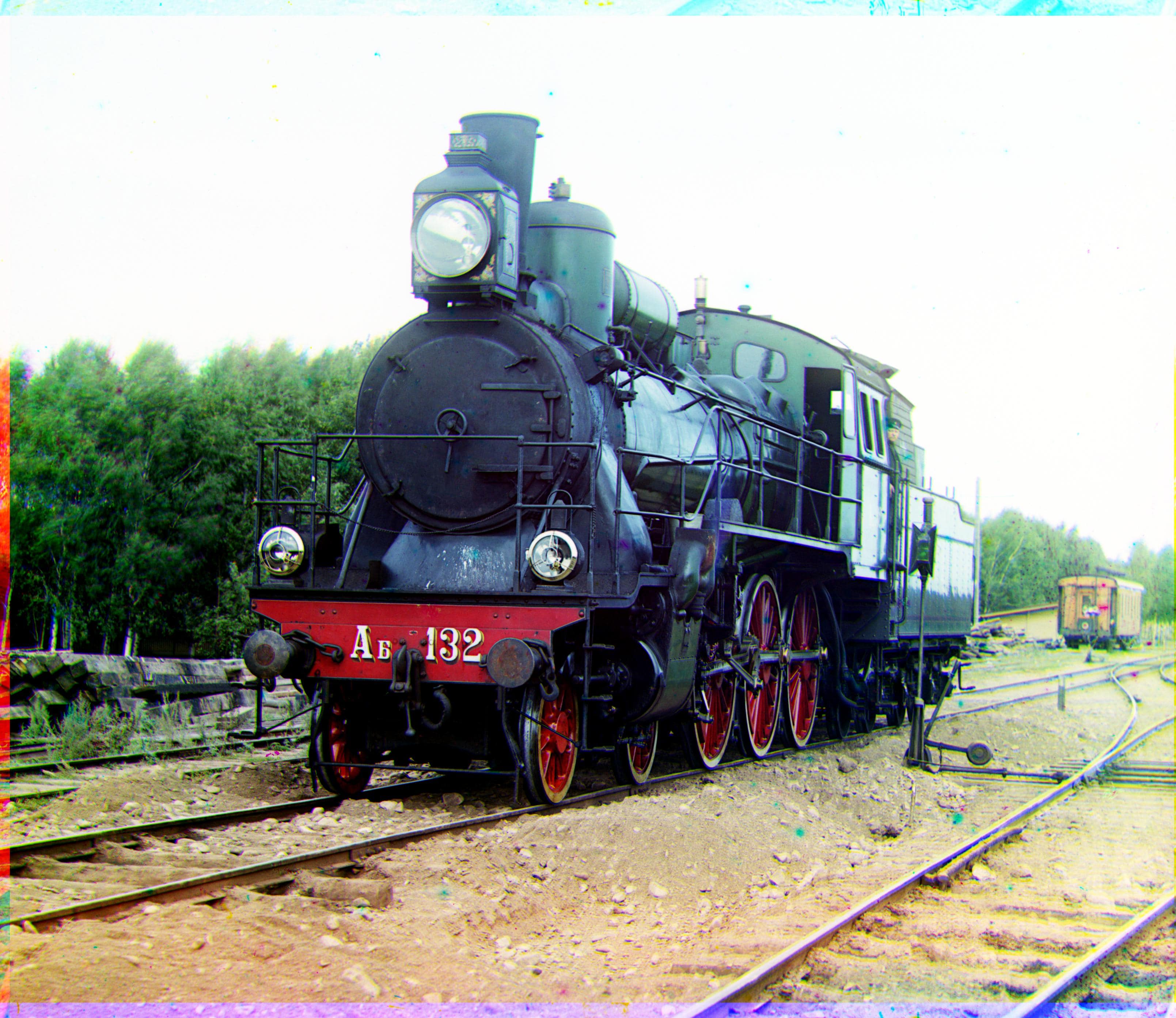
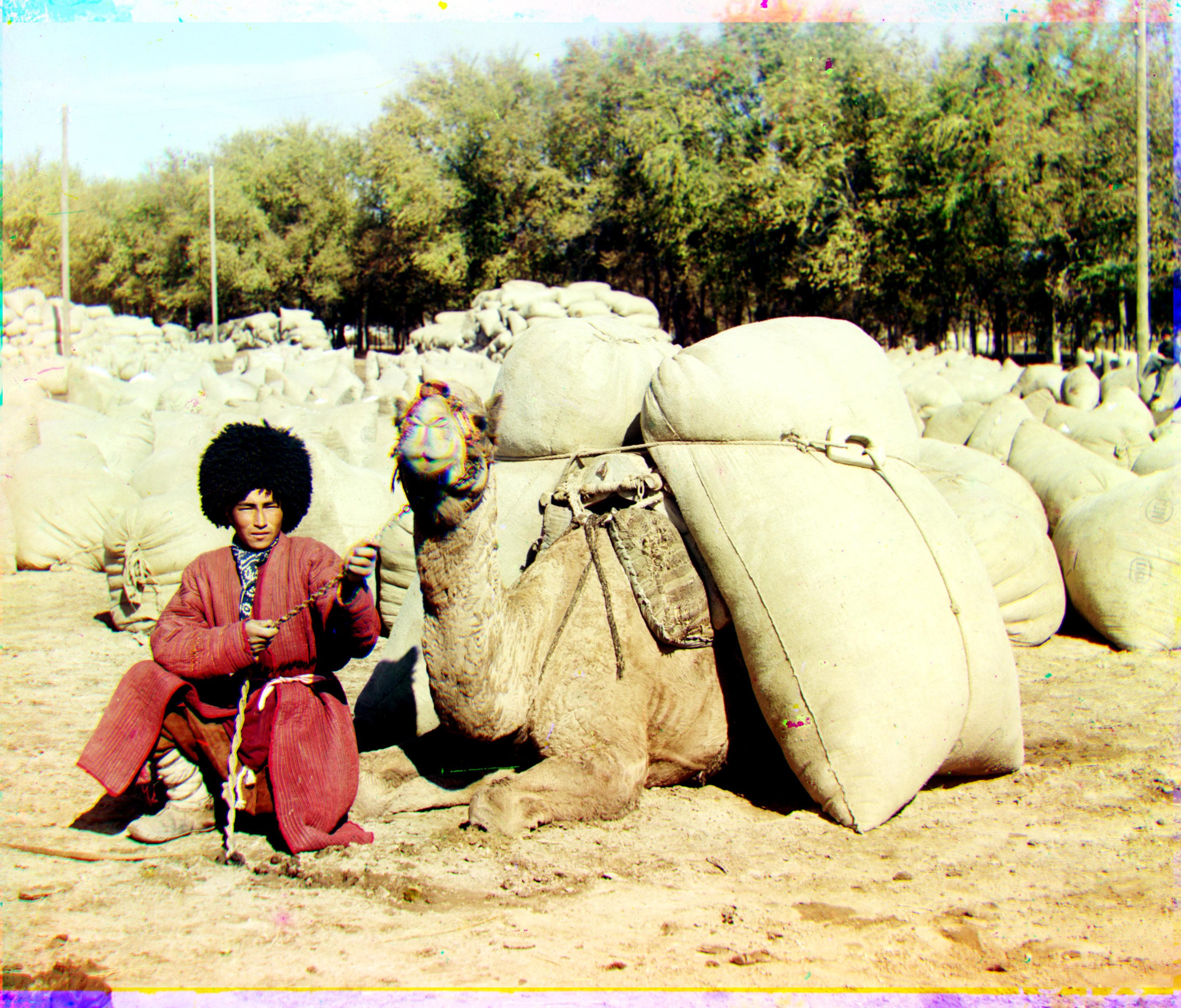
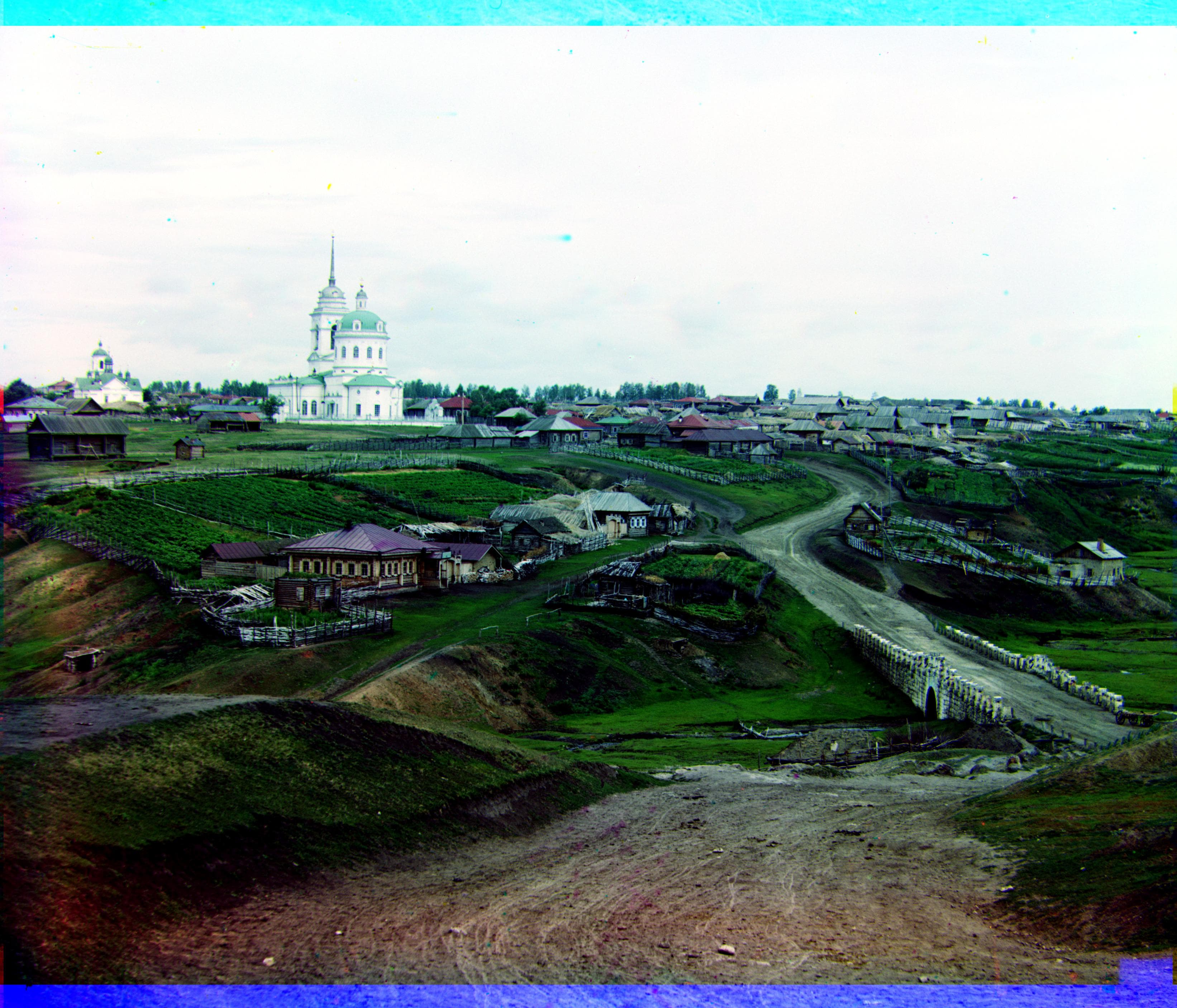
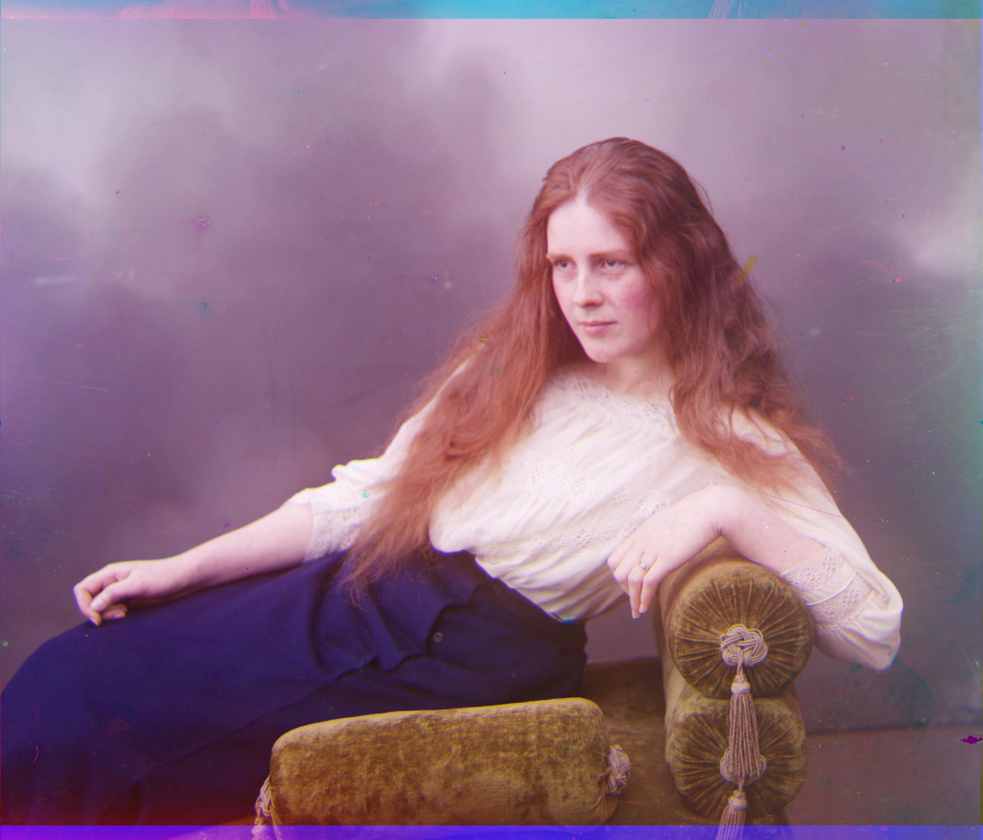
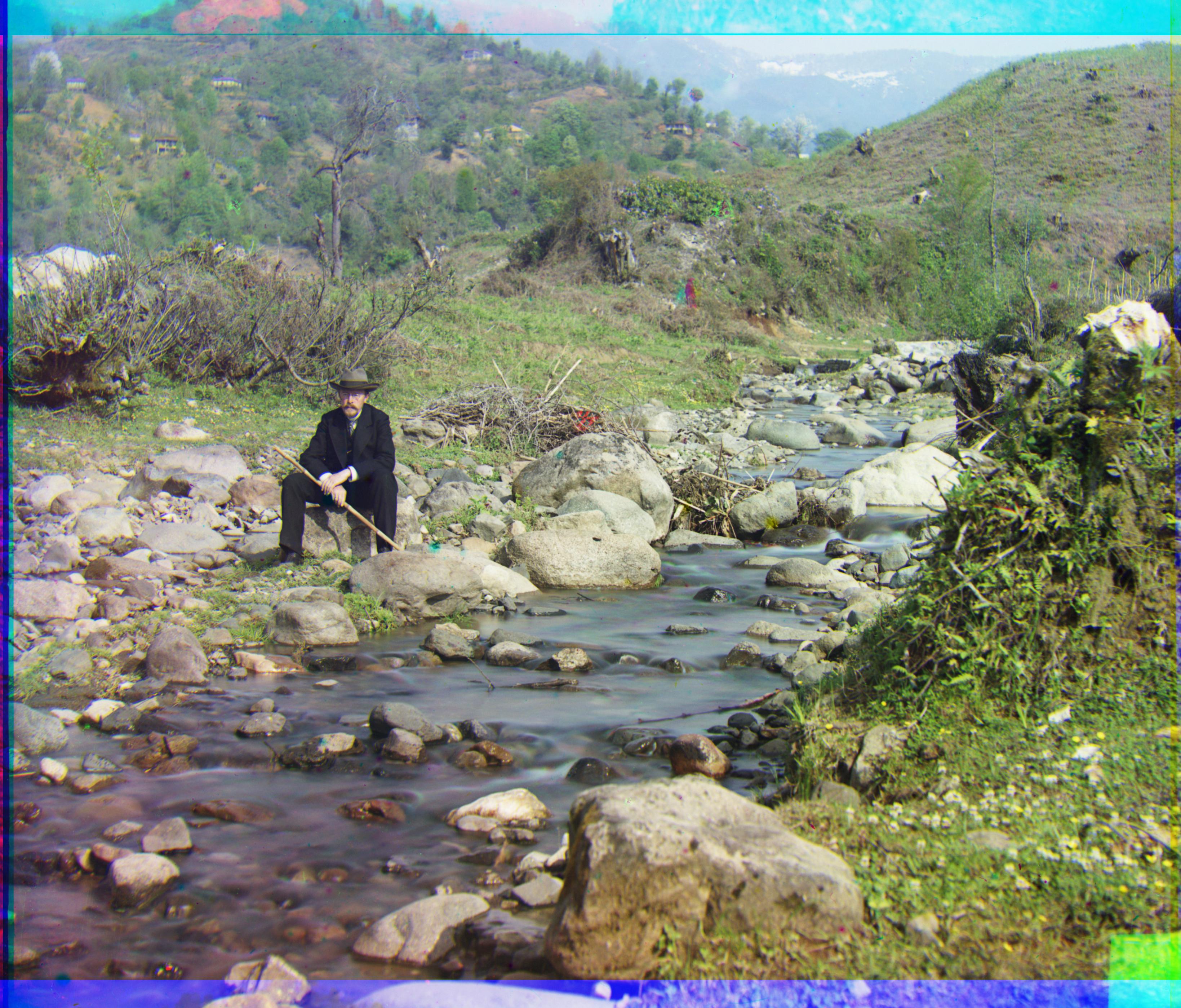
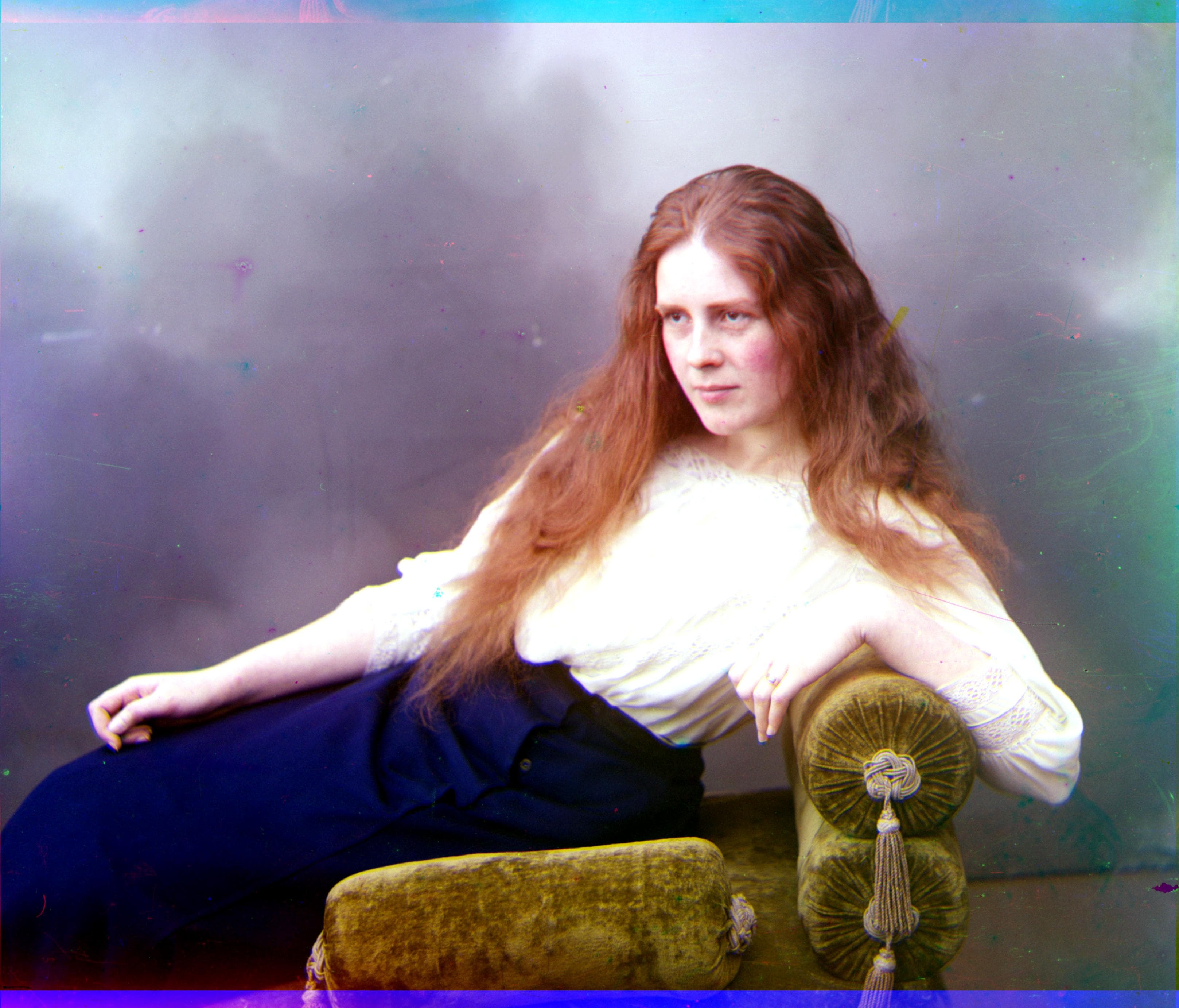
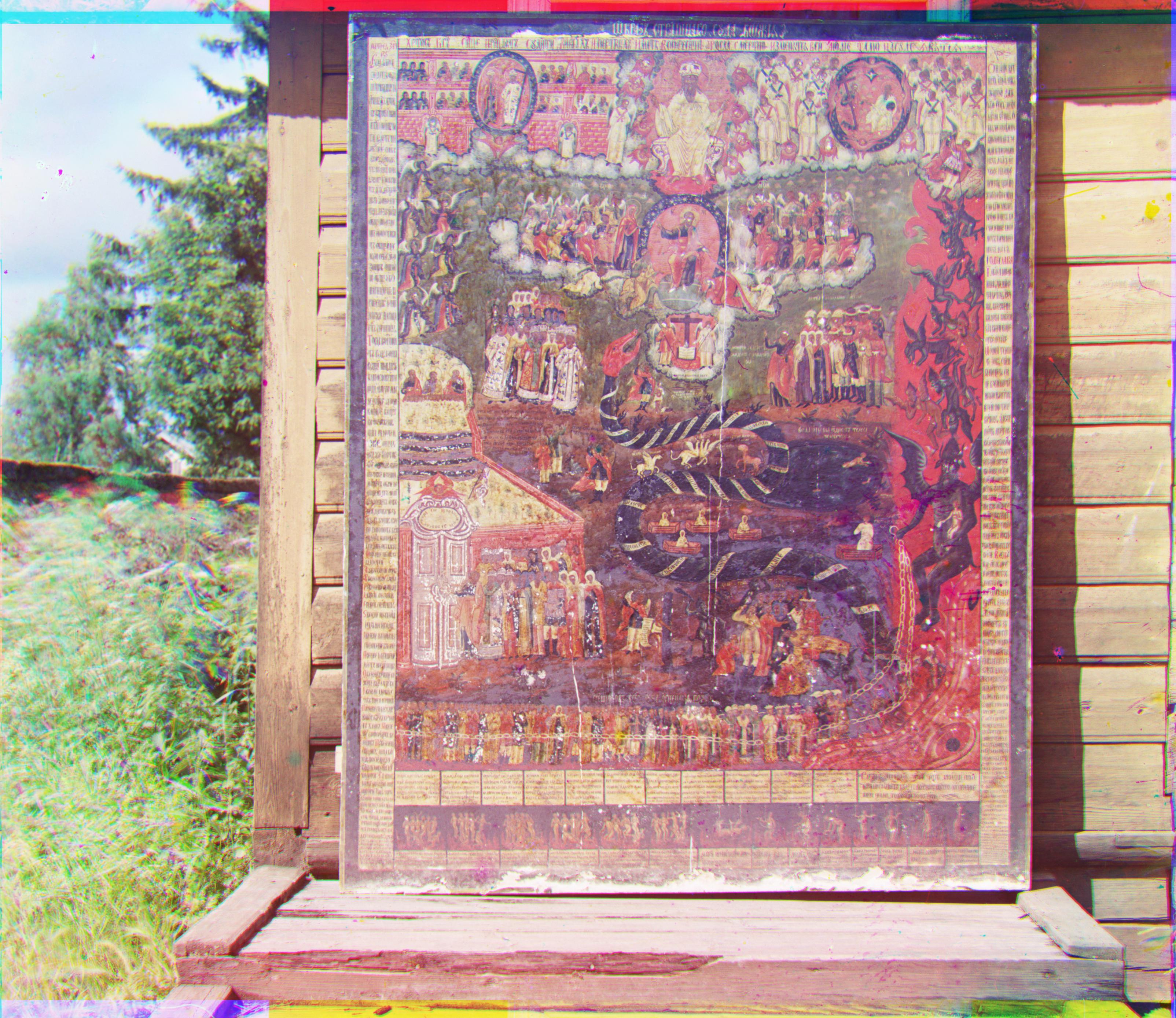
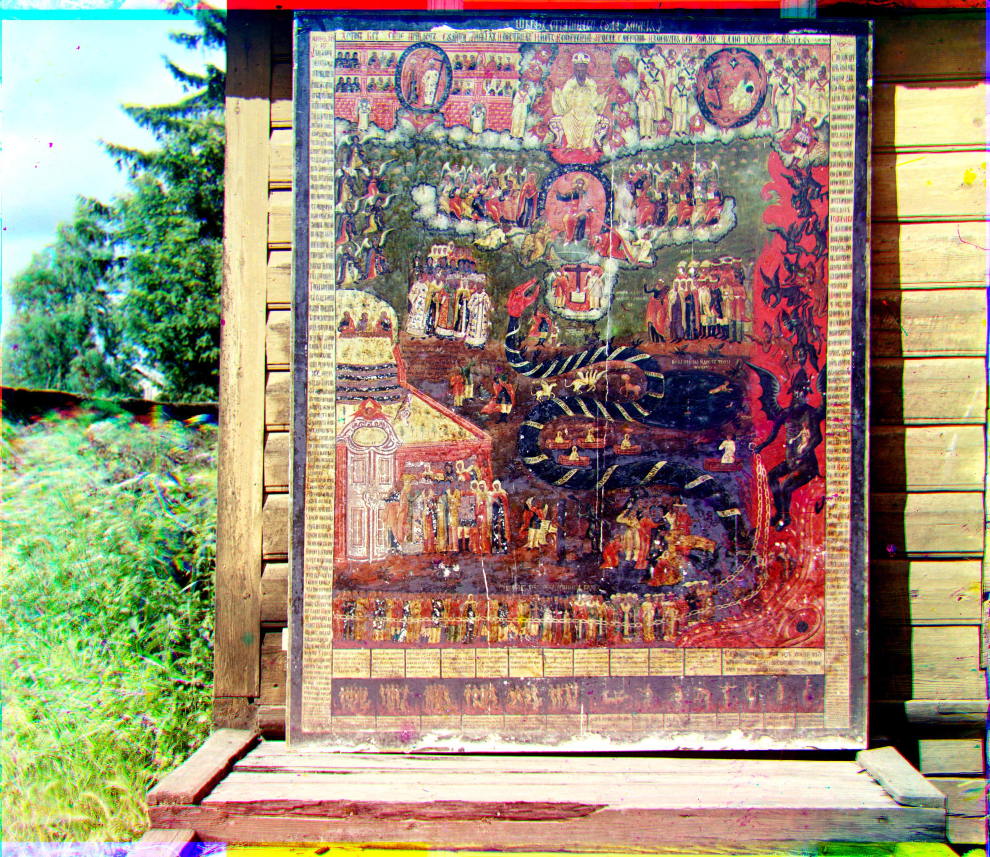
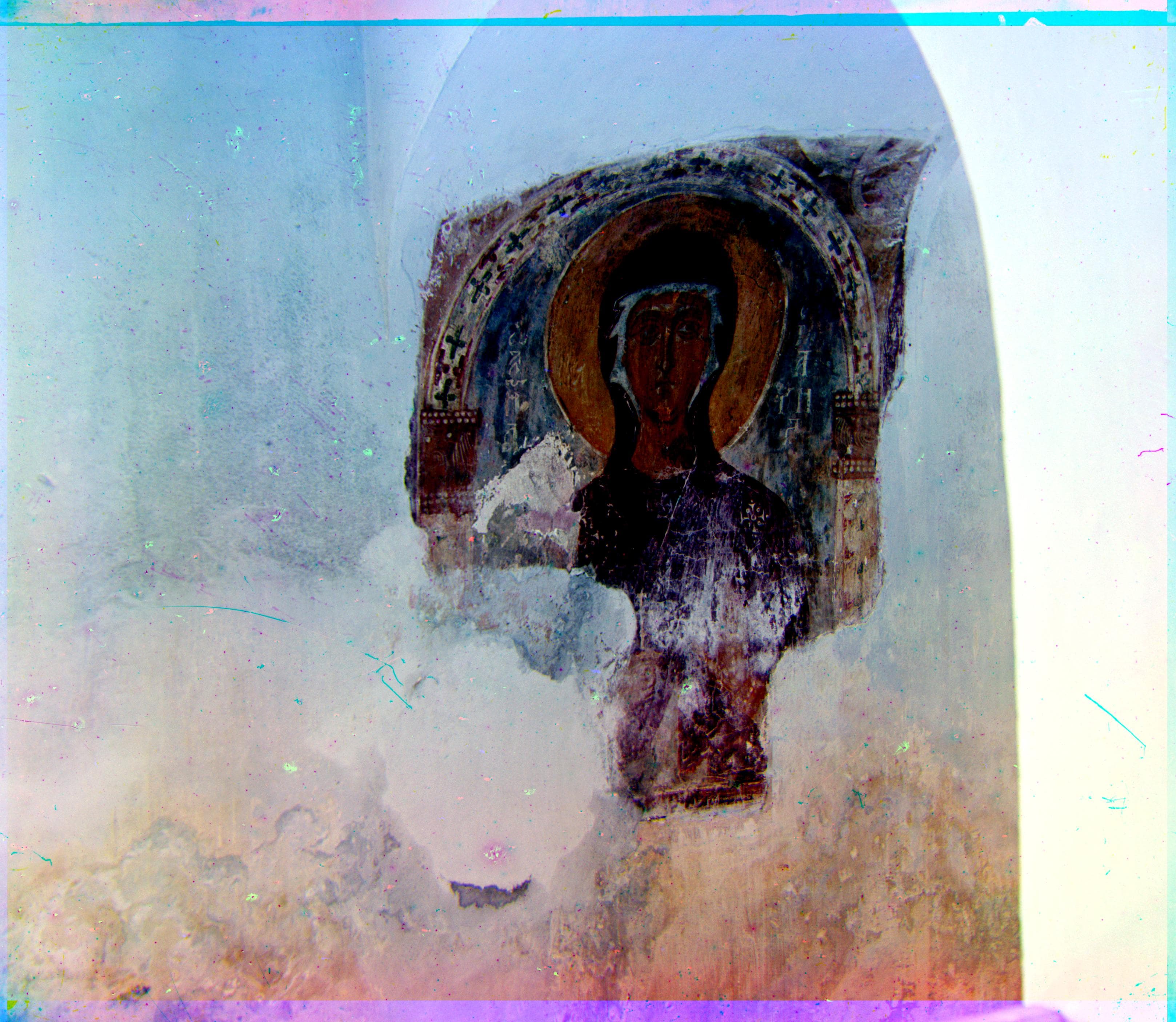
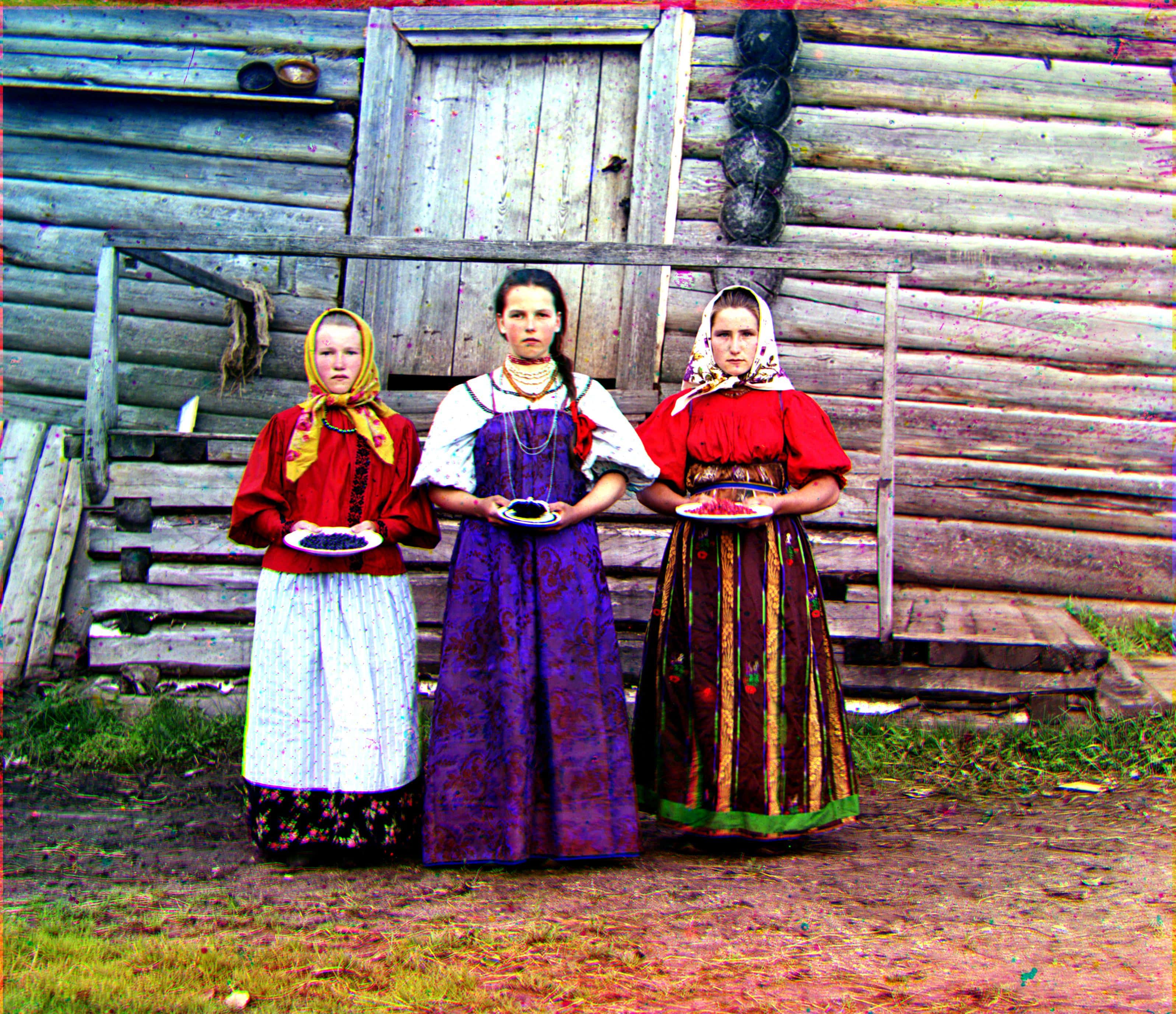
Below are some additional images from the Prokudin-Gorskii collection that I ran my algorithm on!
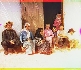
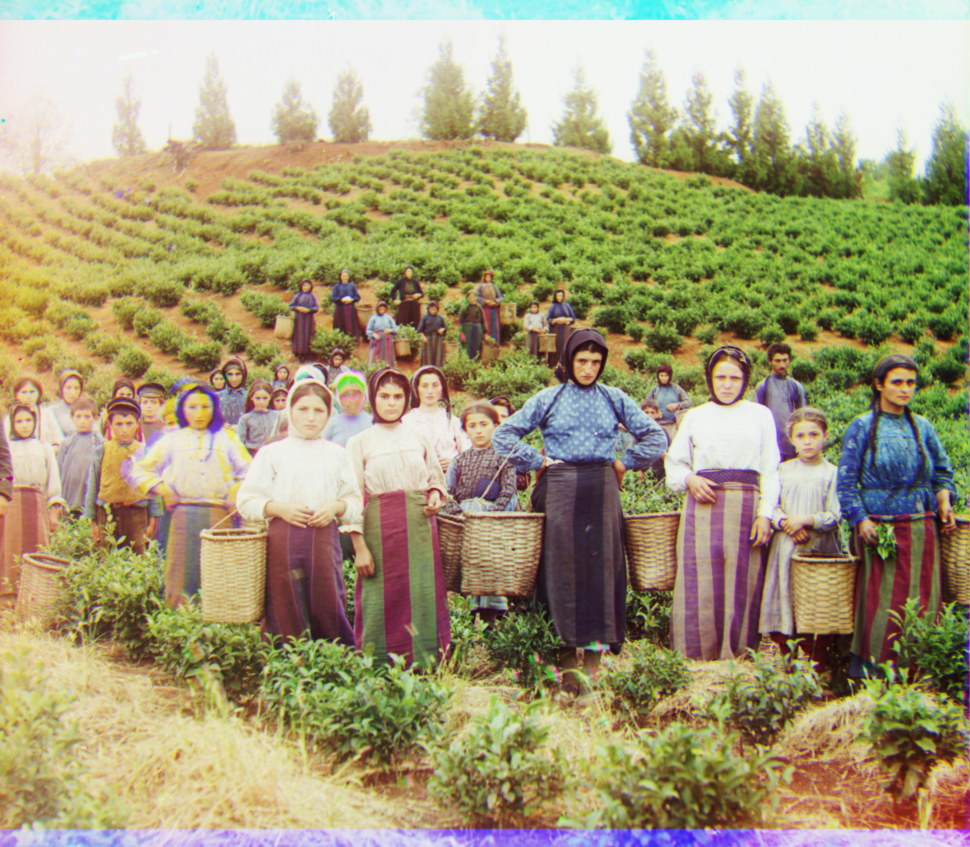
In conclusion, I really enjoyed working on this project, as it was fun to see and learn about how color images are represented and created from distinct red, green, and blue channels. For the most part, I was able to successfully align all the example images given for this project. Some images had a few misaligned areas, such as harvesters.tif, but this was likely due to differences in the composition of each photo- for example, some of the people in the photo seemed to have moved between the different shots, which is why there seem to be a couple people who are of different colors in the aligned image.