CS194-26 Project1: Images of the Russian Empire
Automated colorization of the Prokudin-Gorskii collection
Yao Fu, cs194-26-aen, Fall 2018

In 1948, the Library of Congress purchased a collection of Prokudin-Gorskii’s RGB glass plate negatives, which records three exposures of every scene onto a glass plate using a red, a green, and a blue filter, in order to produce a colored picture. This project aims to use several modern image processing techniques to align the three negatives and reproduce colored images of the Russian Empire at Prokudin-Gorskii’s time.
Alignment
We should first divide each input image into 3 separate parts and then try to align the green (the middle one) and red (the bottom one) parts to the blue (the top one) one. In order to achieve a better alignment, we should get a more accurate displacement. Since the borders of each image are usually very dark and not useful and necessary to align, I just ignore the borders of each image when calculating the displacement. The simple alignment algorithm takes in two cropped images and return the displacement that maximizes the Normalized Correlation(NCC) while limiting the searching range to [-15, 15] pixels.
Other heuristics such as Sum of Squared Differences also works well. This algorithm is enough to produce very good alignment when processing relatively small images.
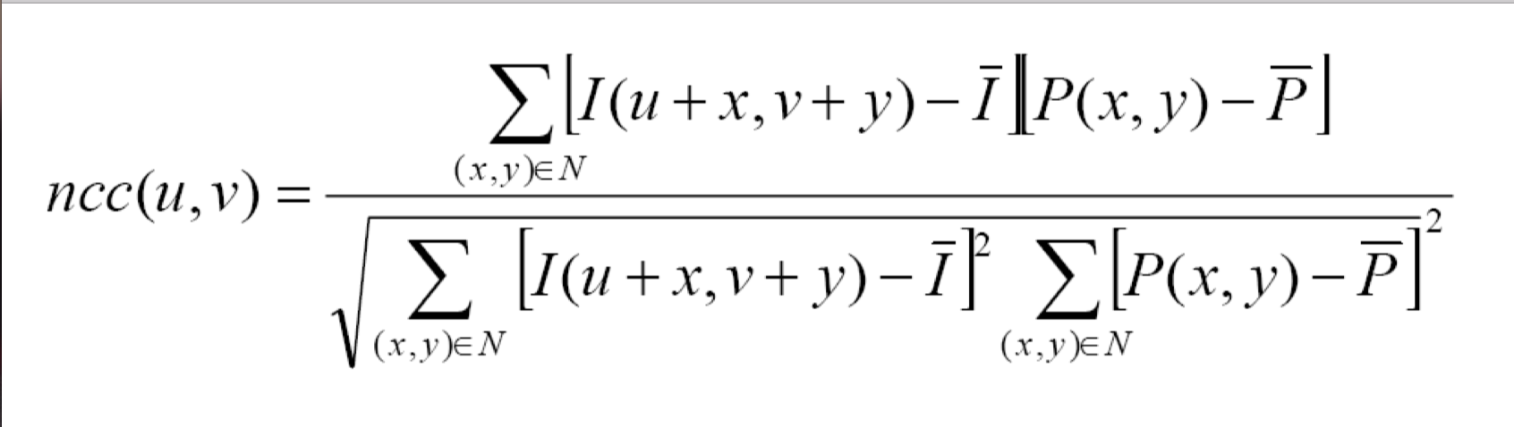
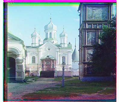
Image Pyramid
However, in order to handle larger images, such as those in .tiff format, we should speed up our algorithm. Also, a displacement in [-15, 15] is not enough at all to overlap two 3000*3000 images. Thus, building an image pyramid is a good choice here. While the size of an image is too big, we calculate the displacement of a coarser version of this image (1/2 * 1/2 = 1/4 of the original size) and rescale the displacement by 2 to get an estimated output. An adjustment value can also be calculated on a small portion of the image and added to the scaled displacement to achieve better performance. Applying this algorithm enables processing the .tiff images in within 20s, which is much faster than the original method (several minutes).


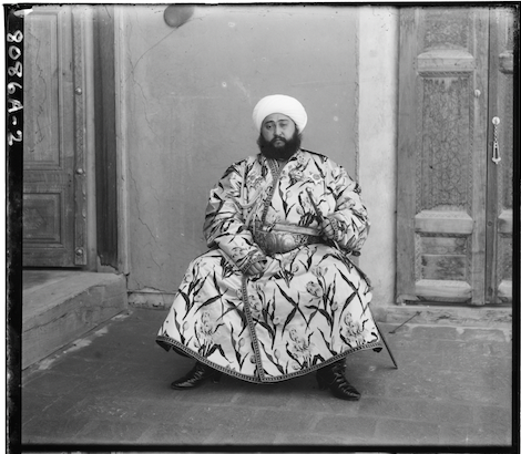
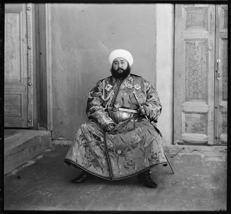
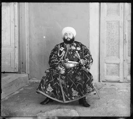
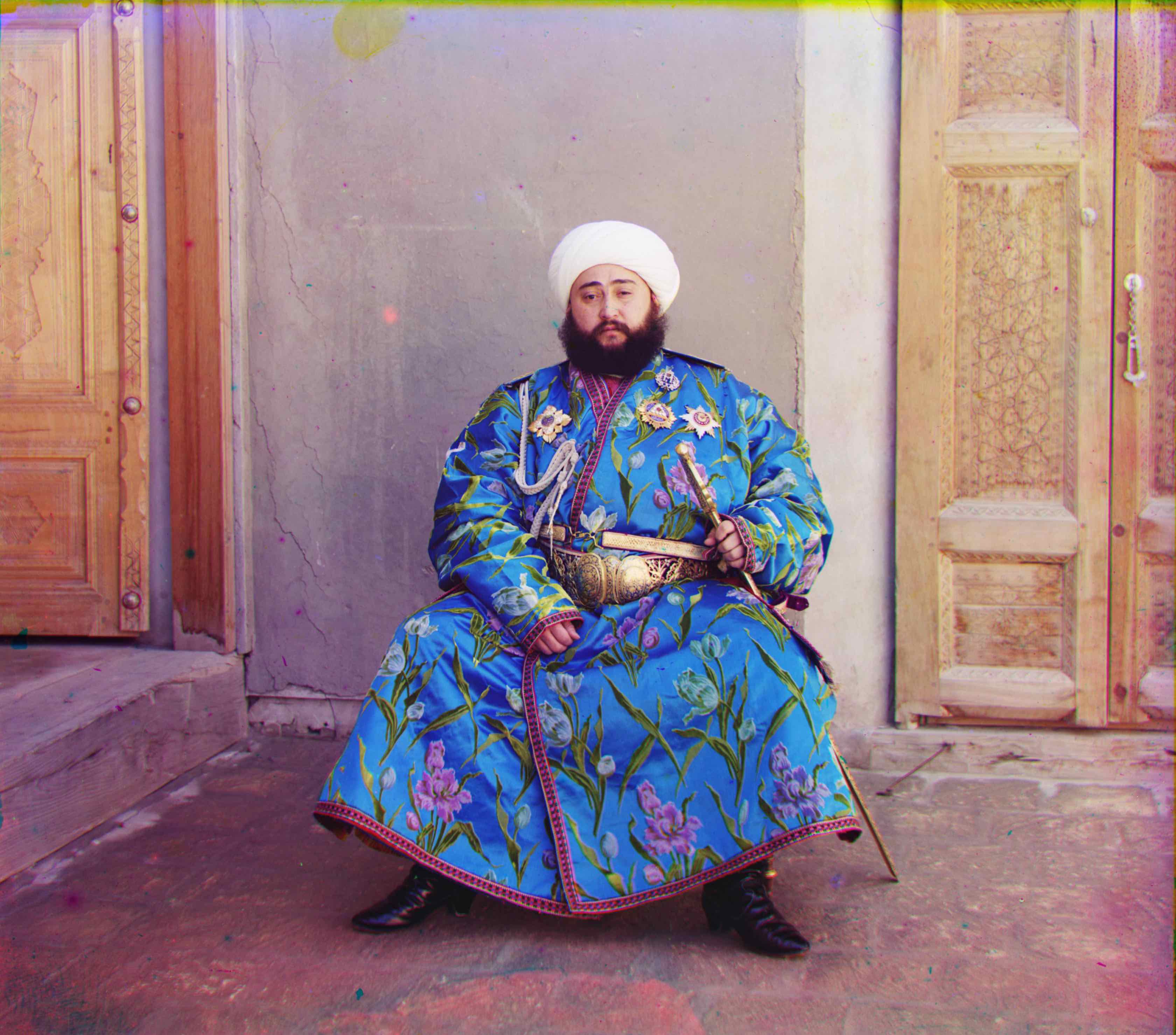
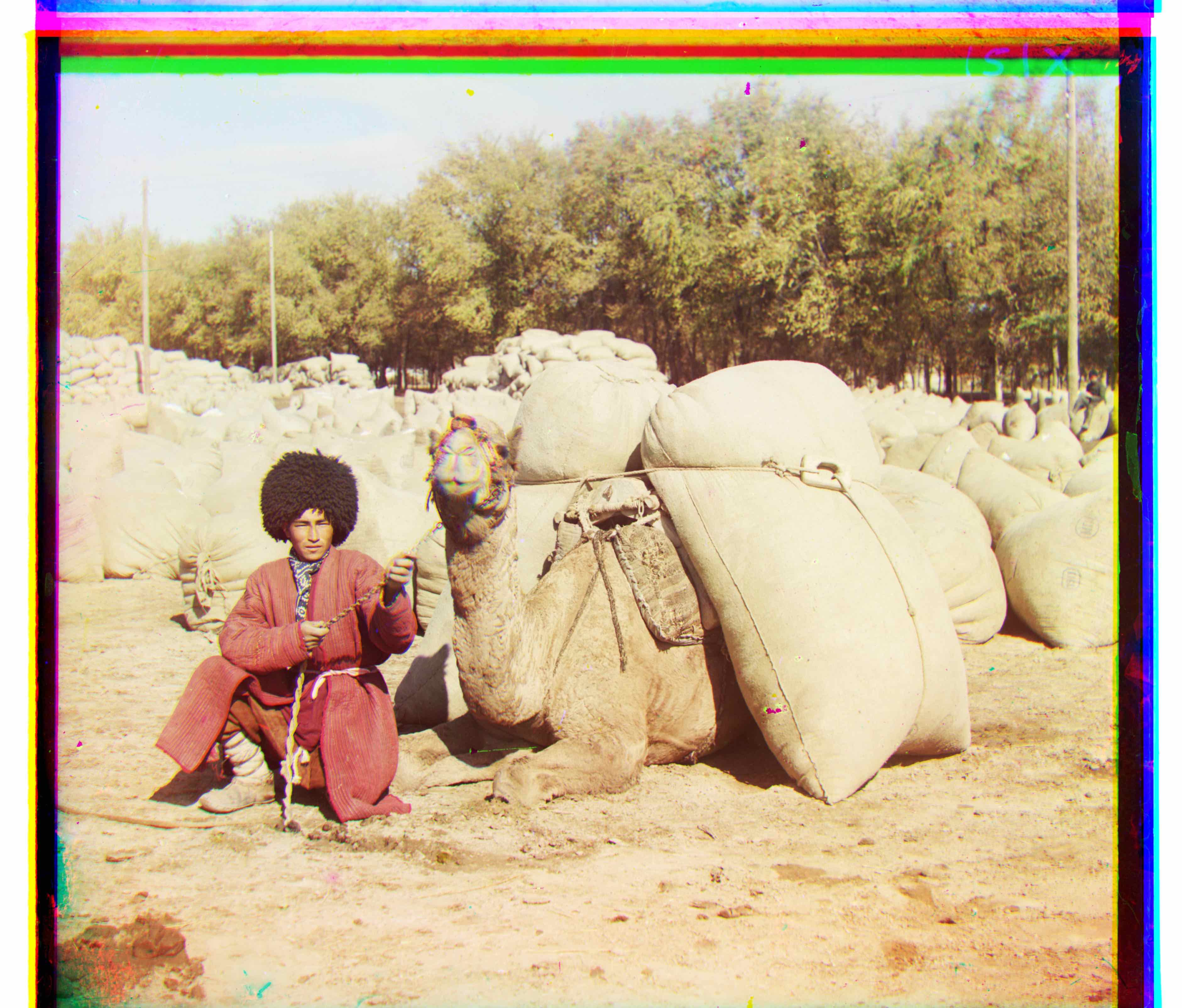
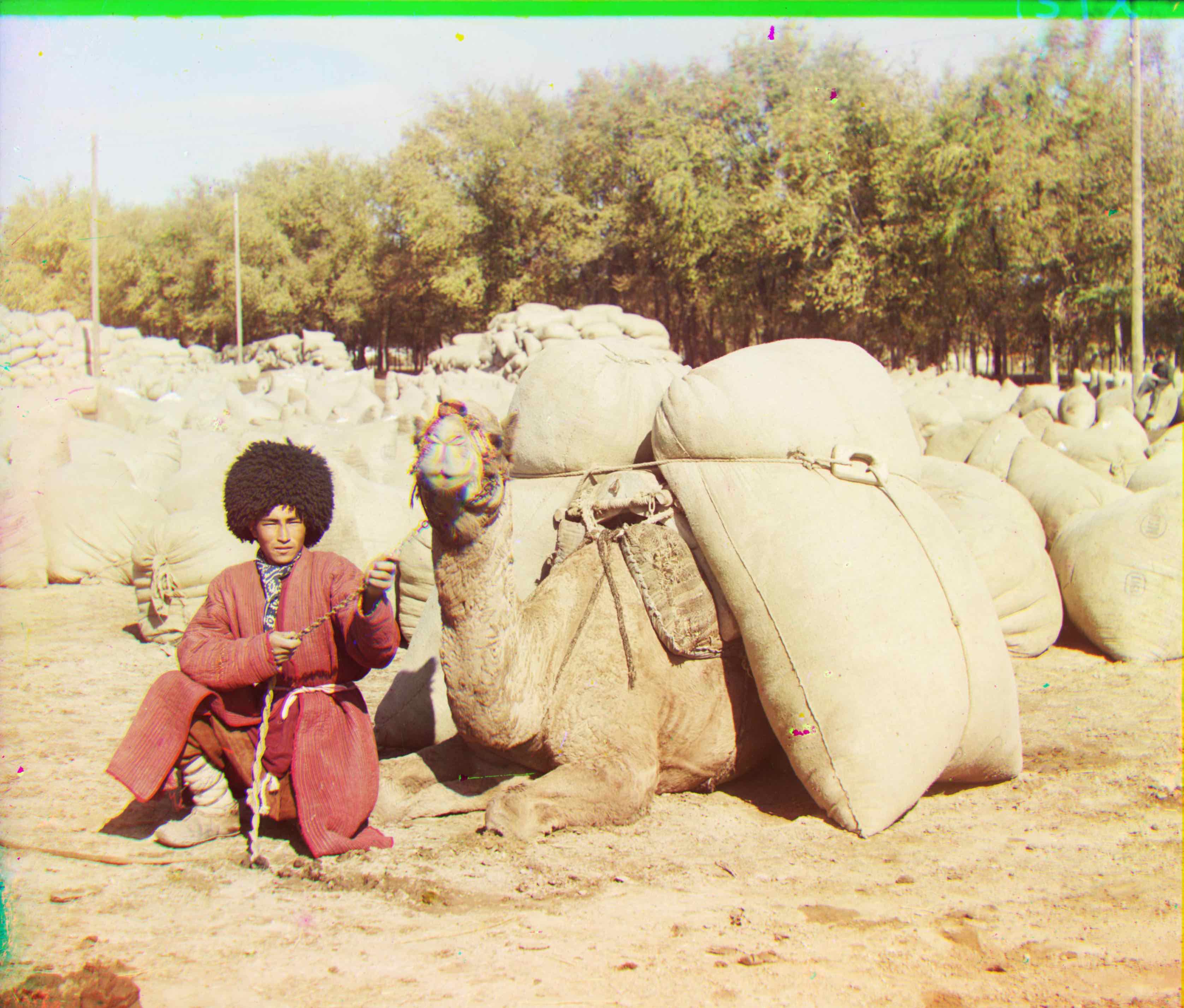
Now that nearly all the images aligns pretty well, except the emir one, maybe for the reason that the color contrast in this picture is more sharply than other pictures so the 3 colors have very different densities at the same point. Therefore we should consider other aspects instead of just RGB similarity when aligning.
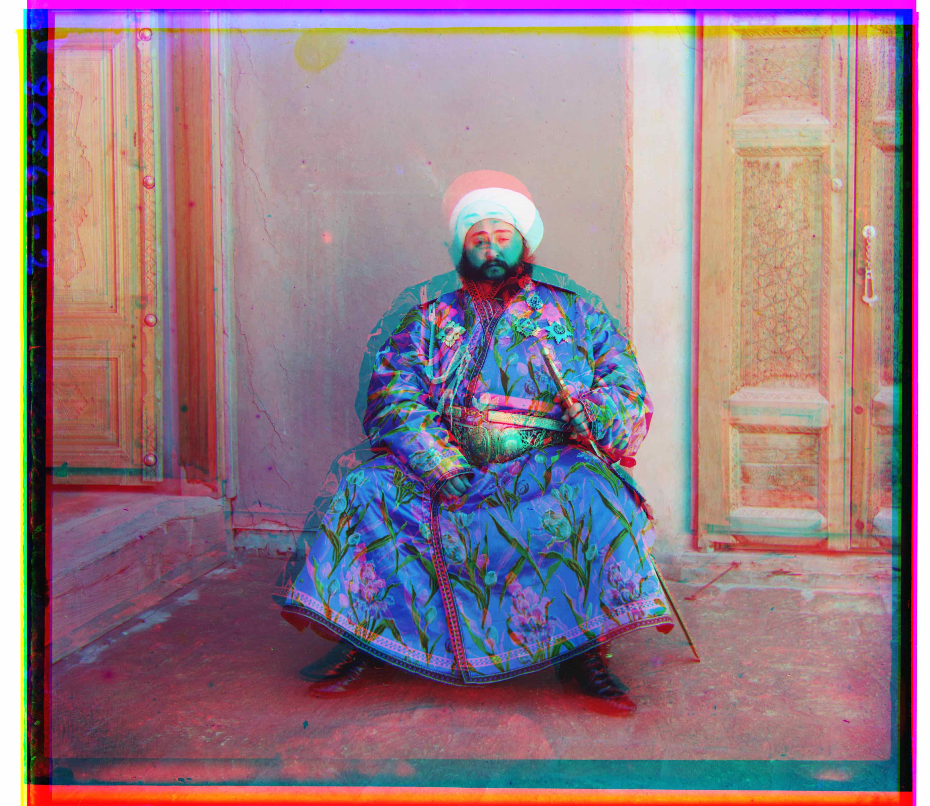
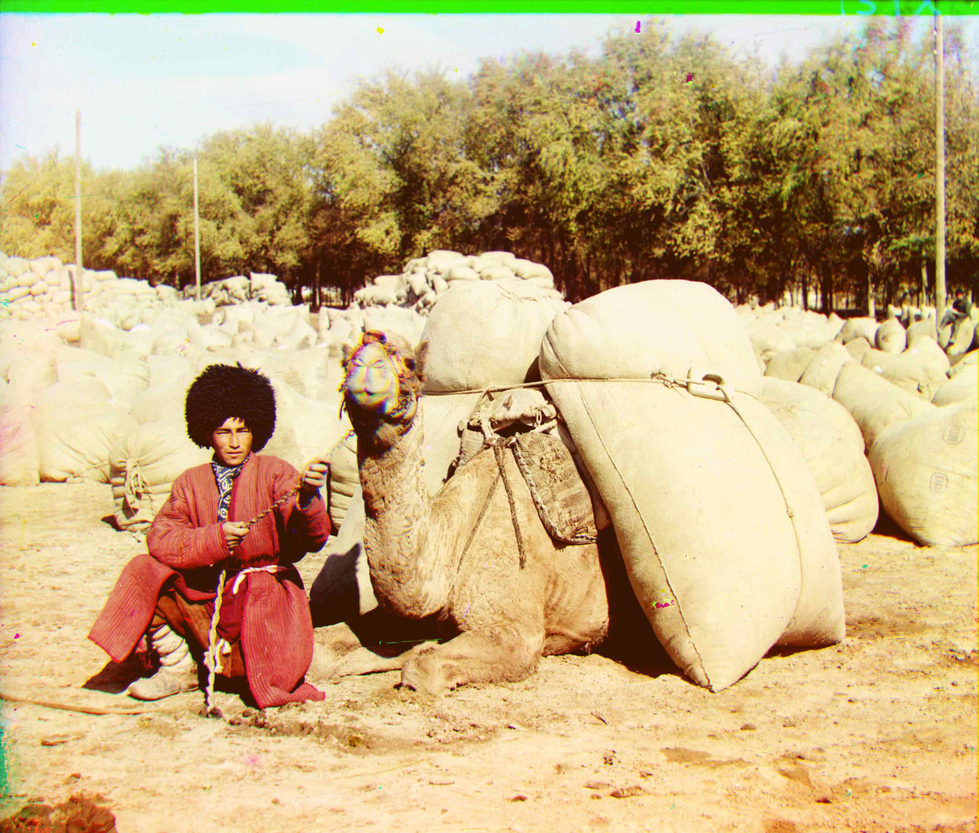
Emir
16.64484 seconds
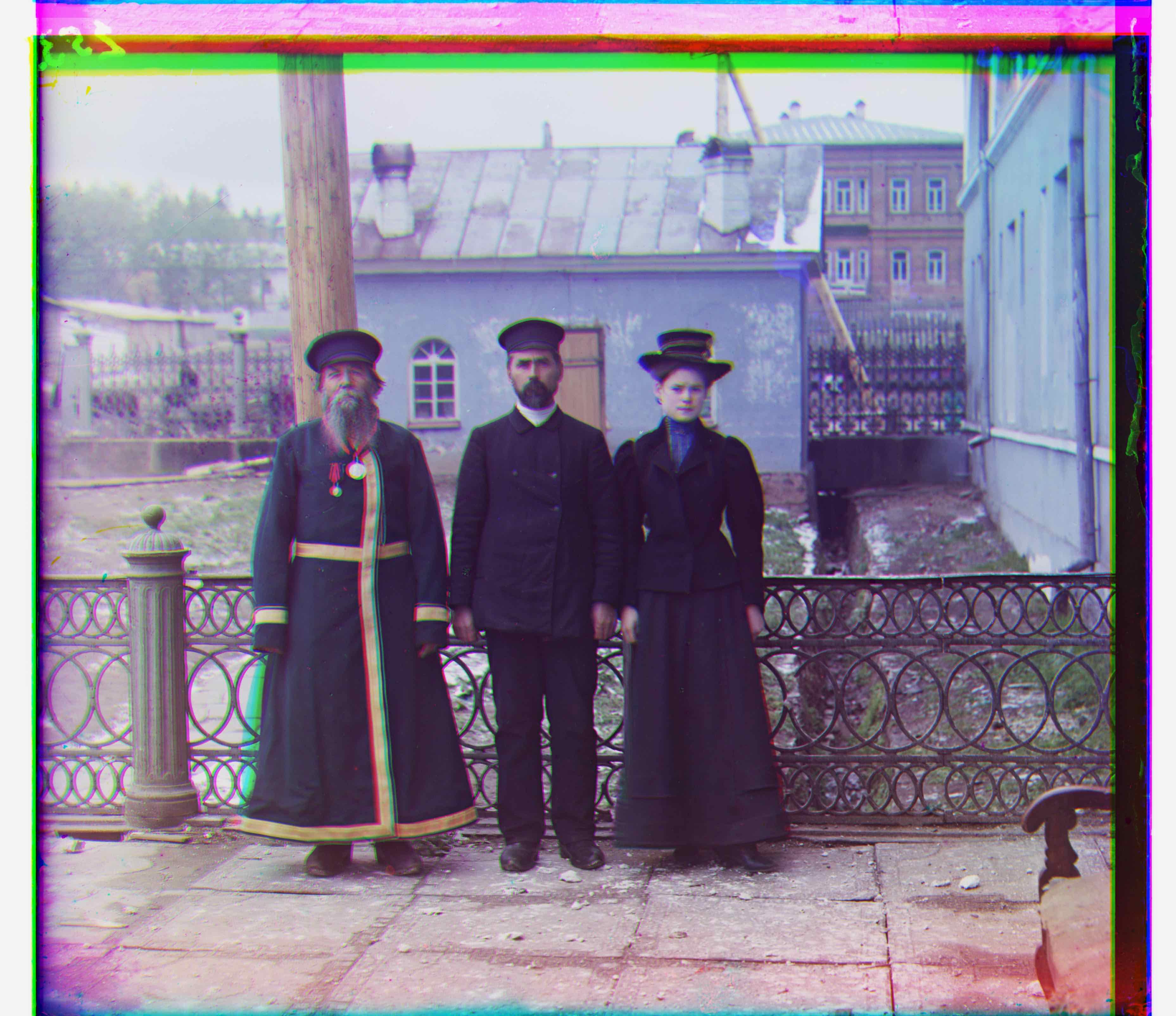
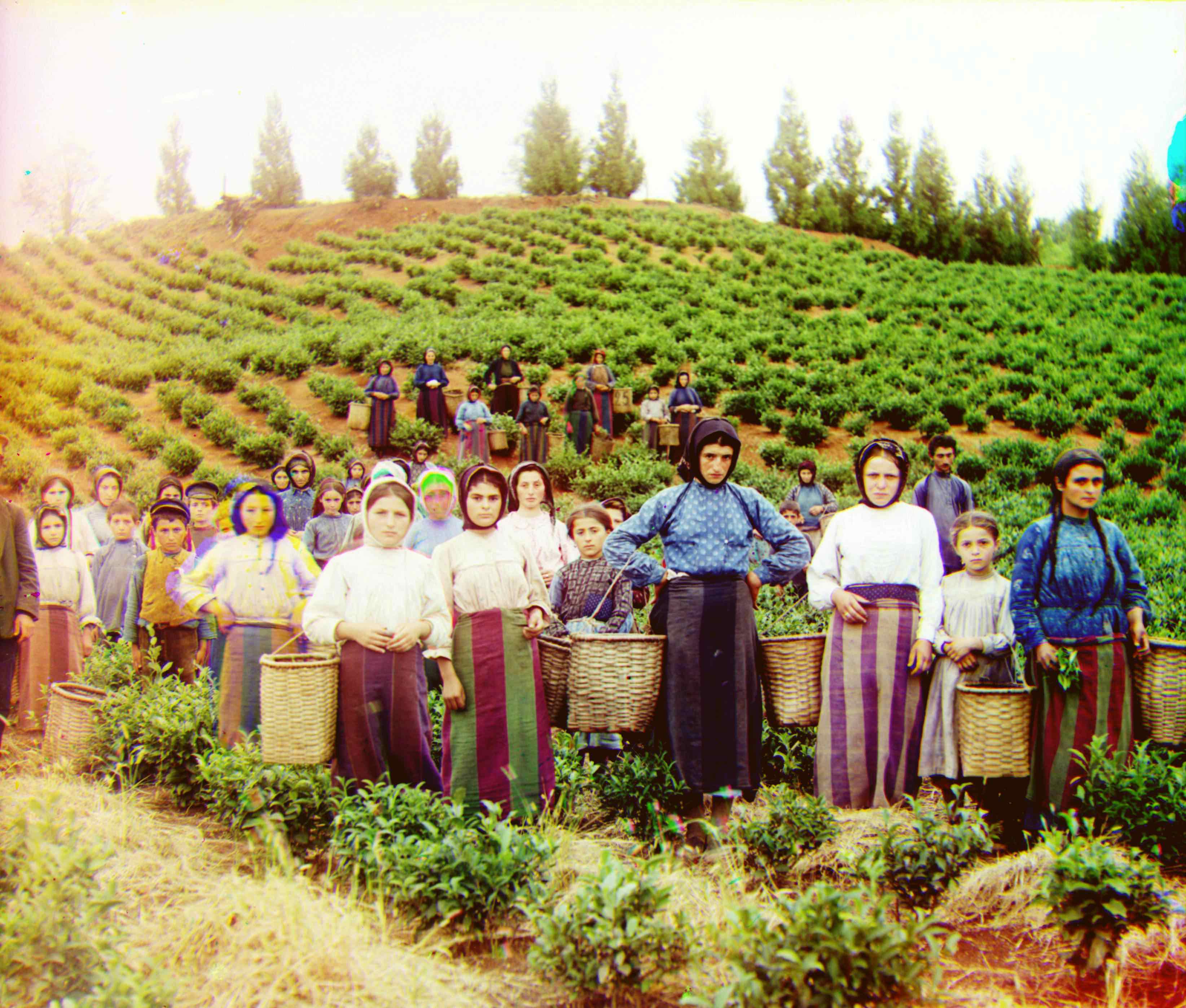
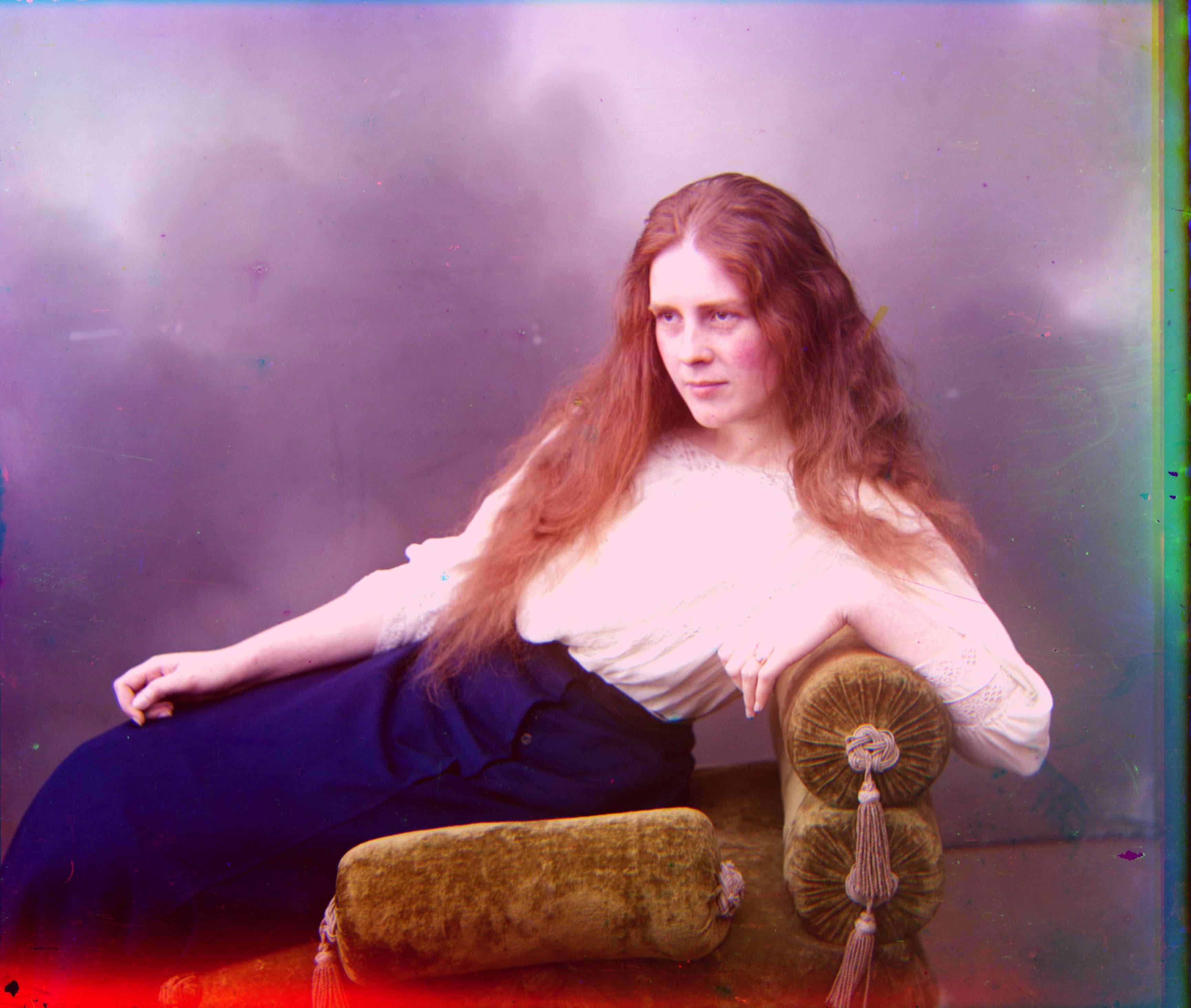
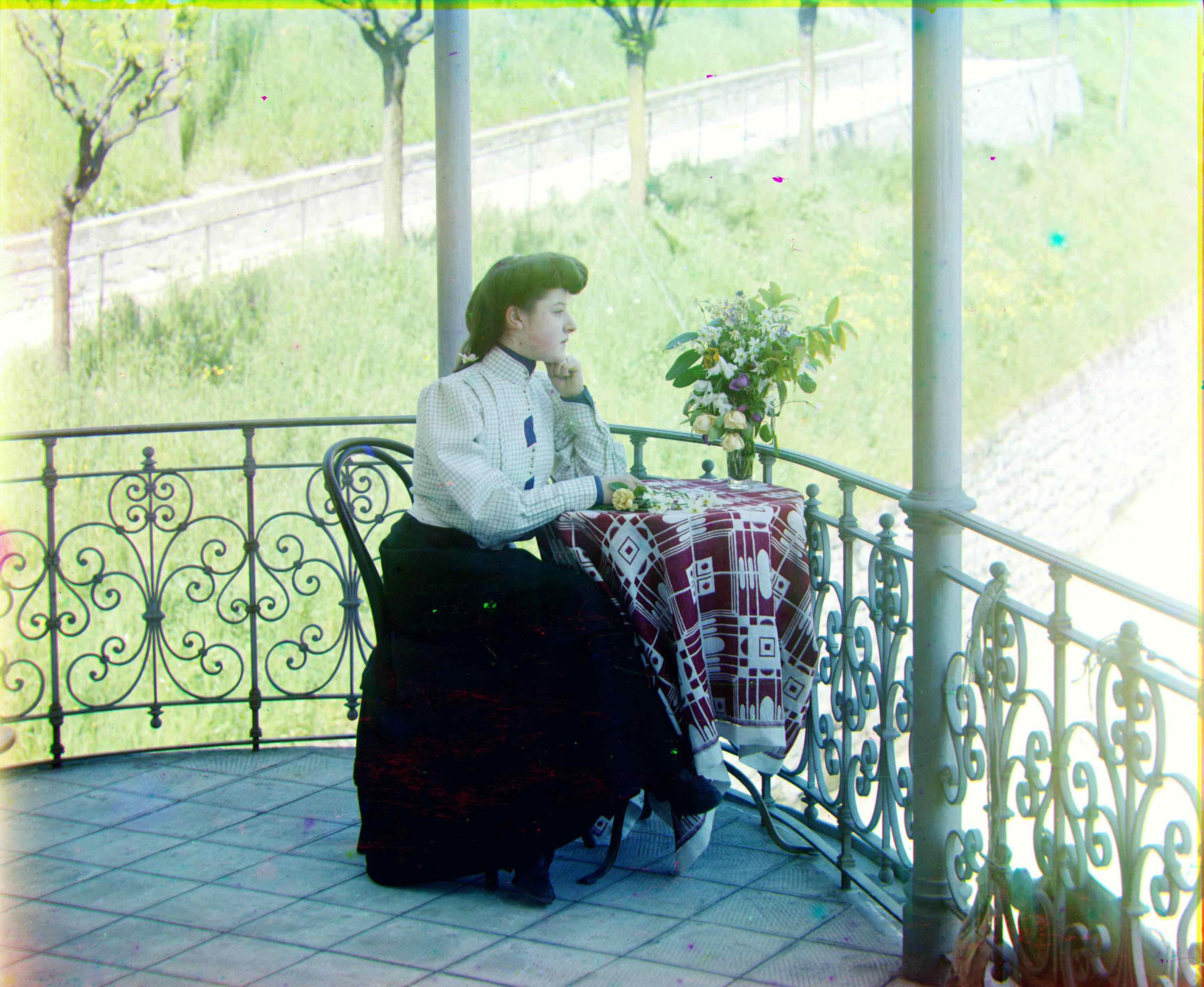
lady
17.942198 seconds
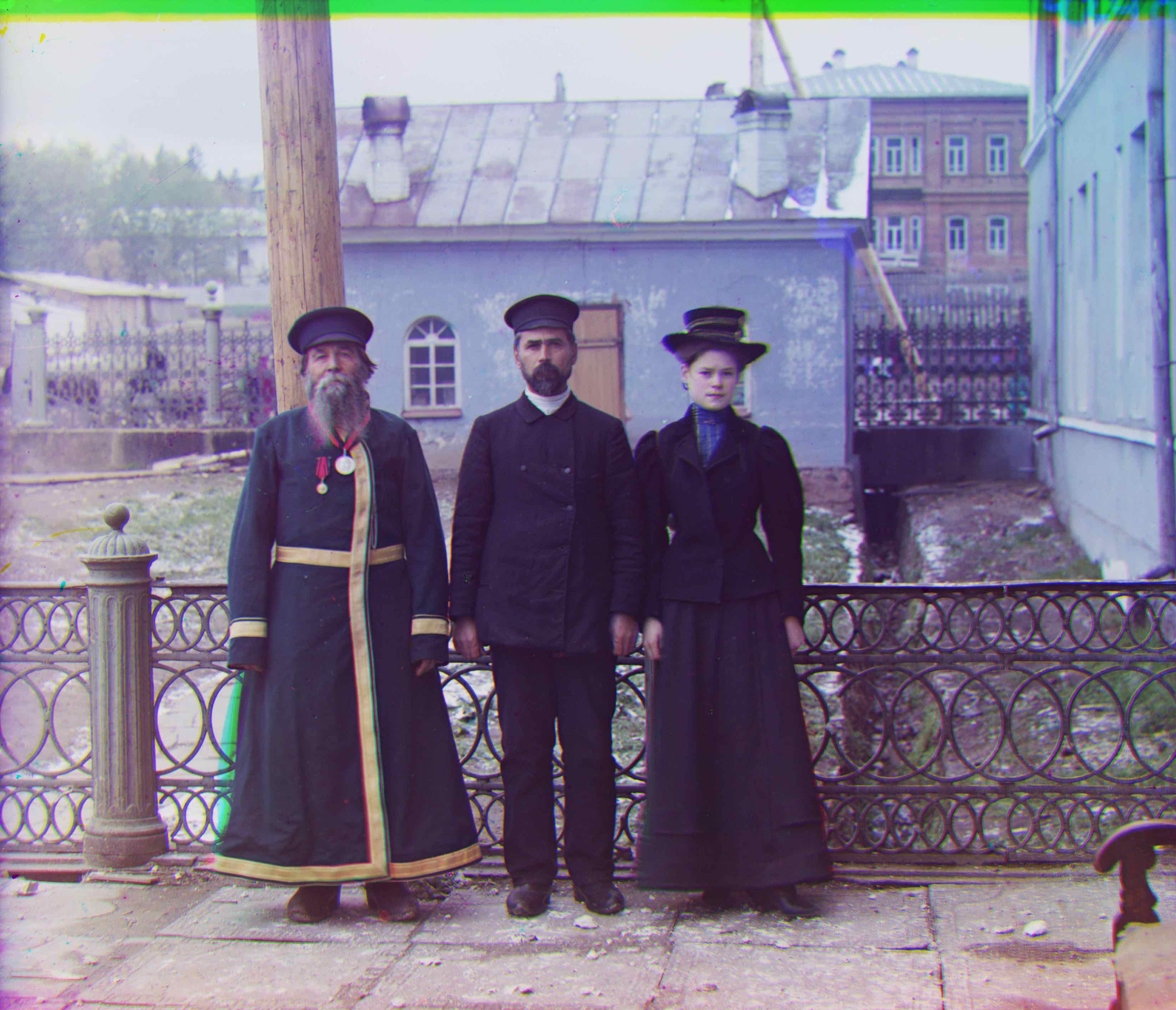
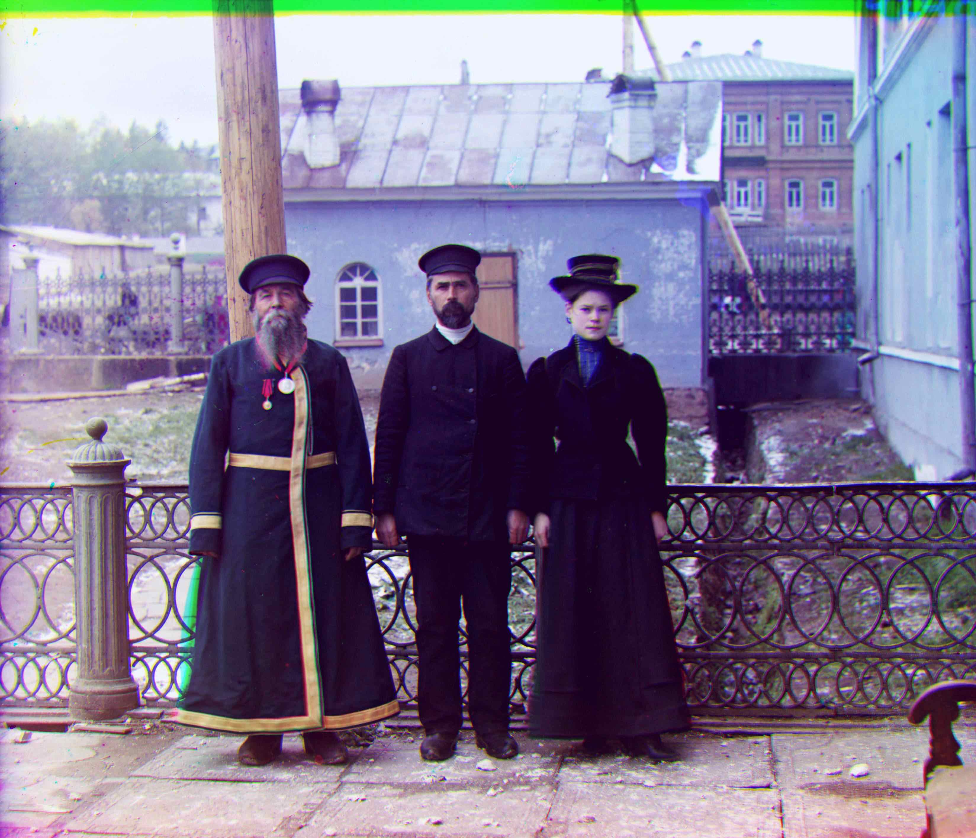
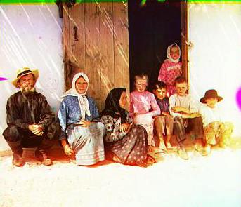
three_generation
18.35918 seconds
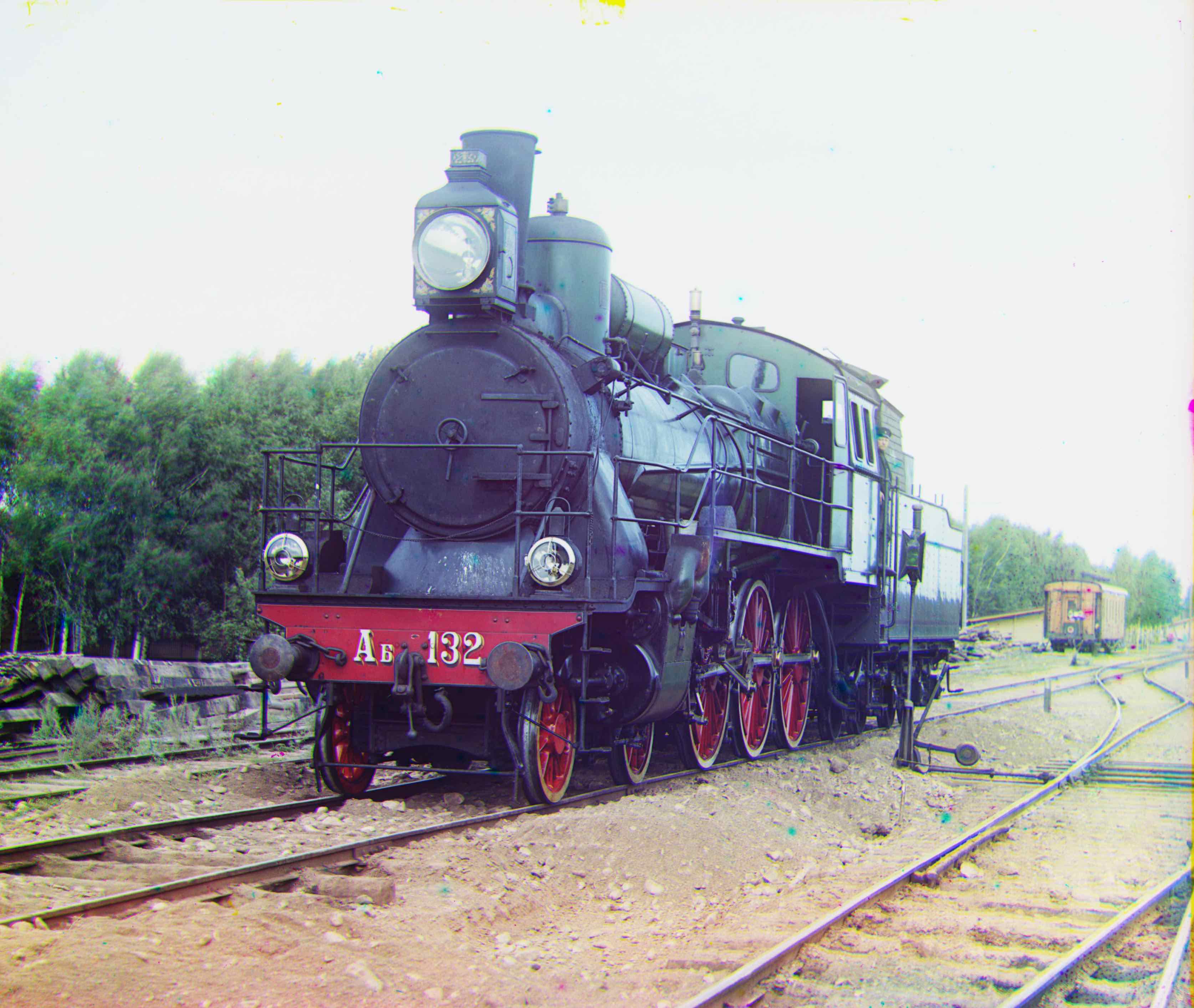
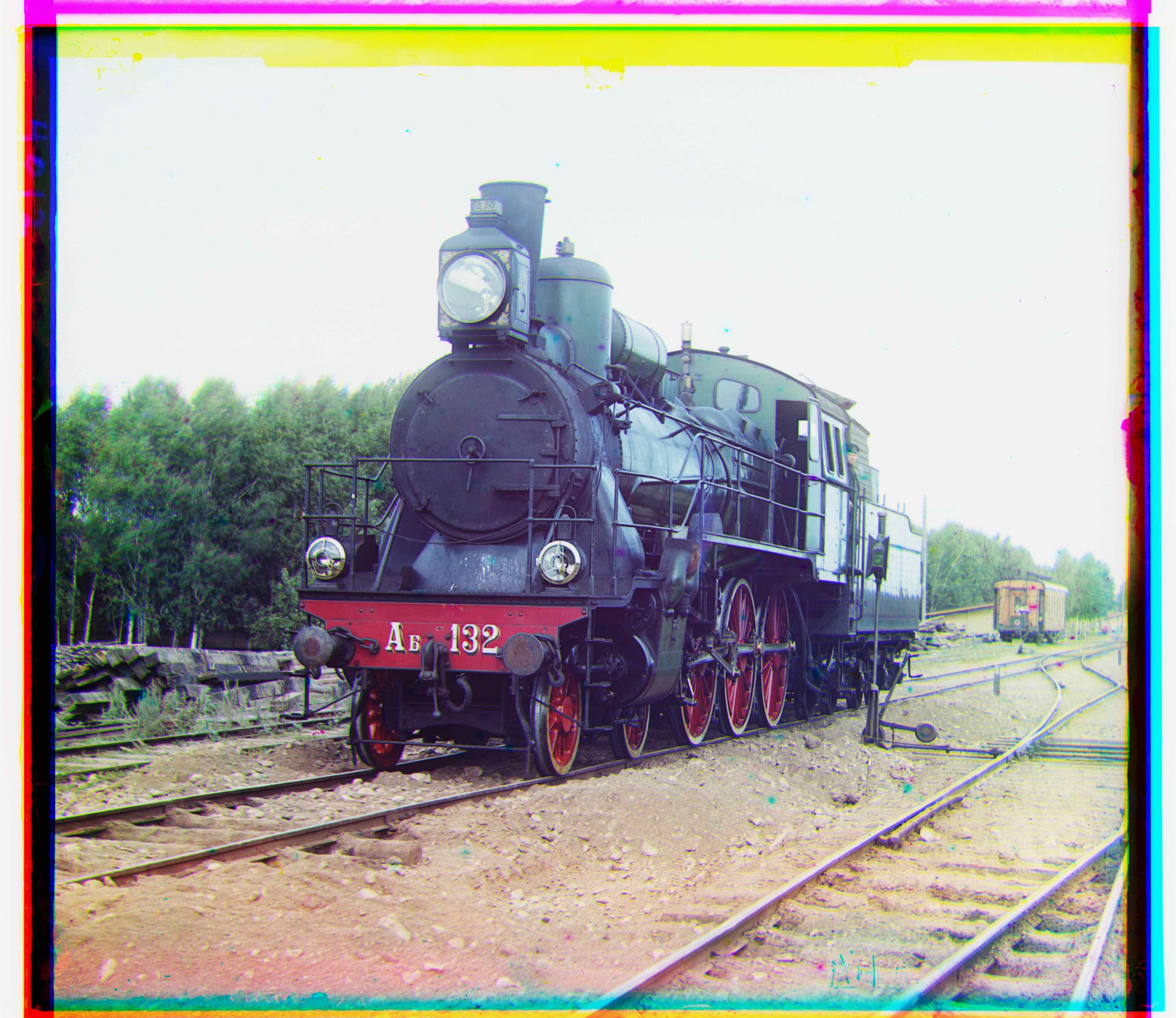
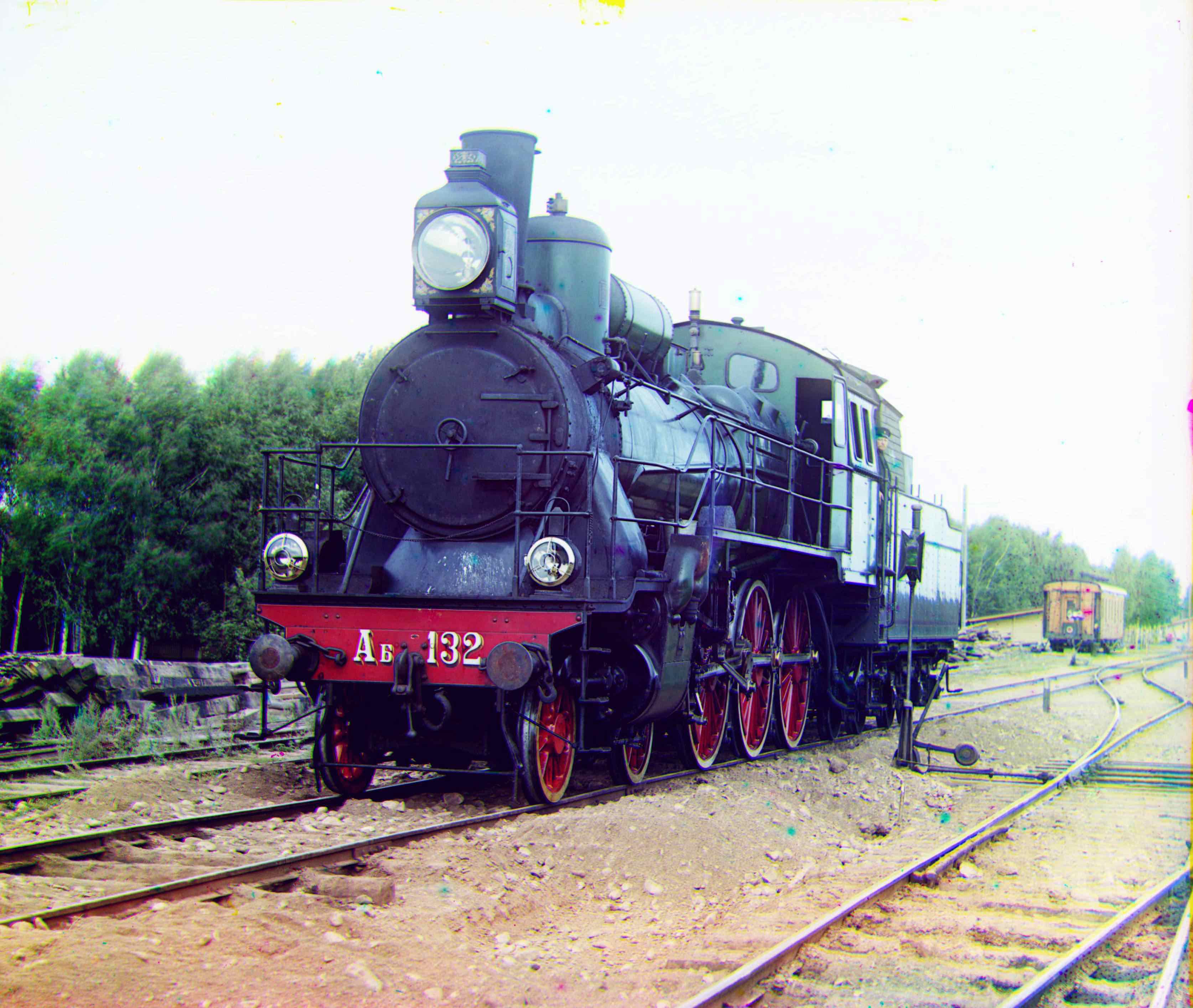
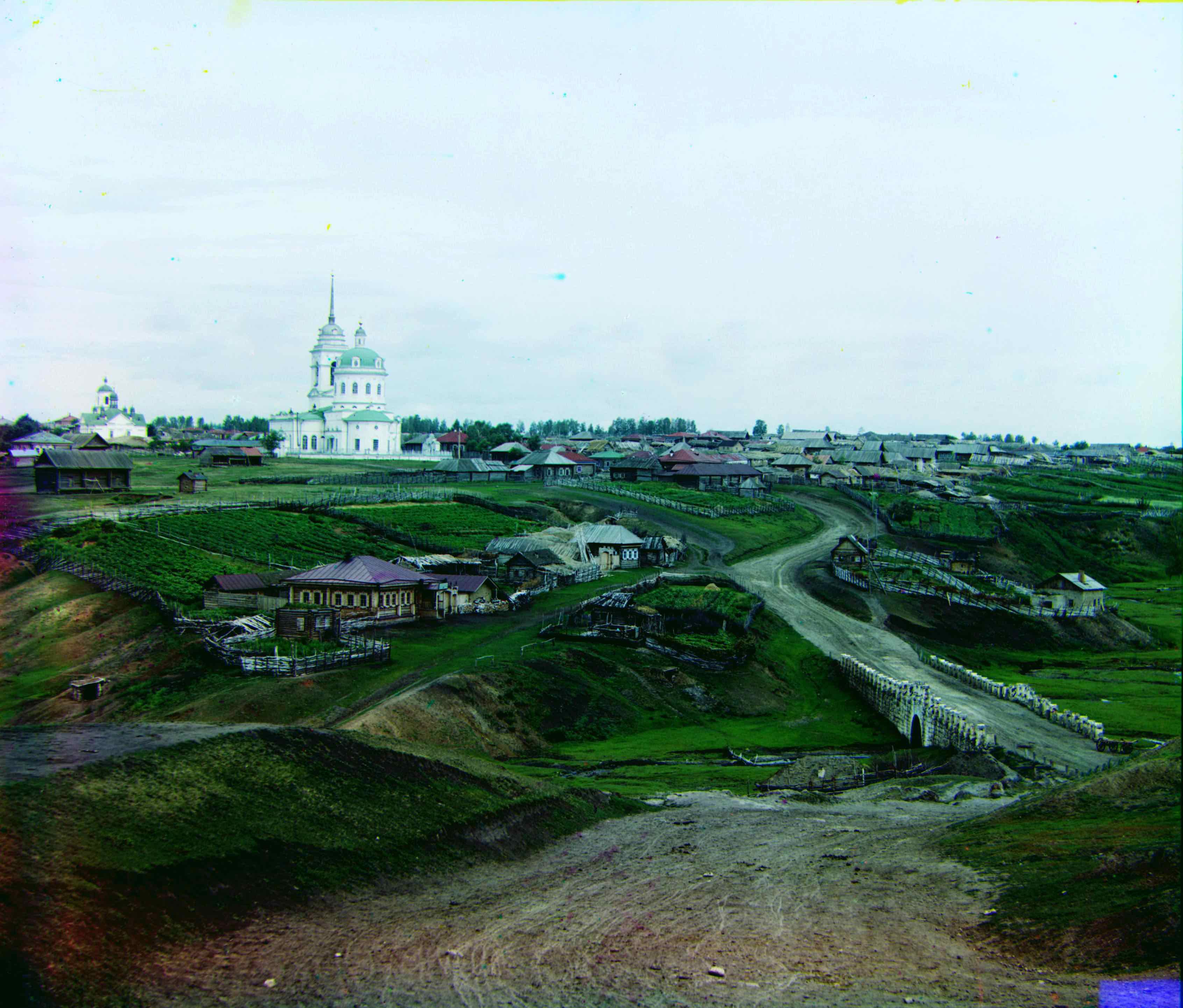
train
17.83017 seconds

Bells & Whistles
Edge detection
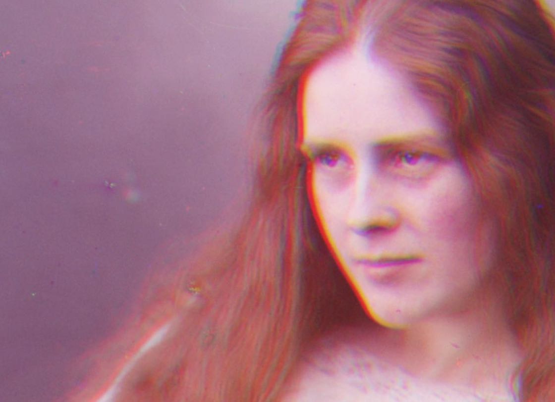
Edge detection turns out to be a good substitute to the previous method. I simply choose Canny Edge Detection to produce a black and white version of the original image and use it to calculate the displacement instead. Although the detected edges are not as satisfying, it still improves the alignment greatly. But there is also drawbacks: I just found that the lady one becomes slightly blurrier now. All others seems to be good enough.
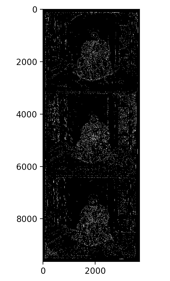
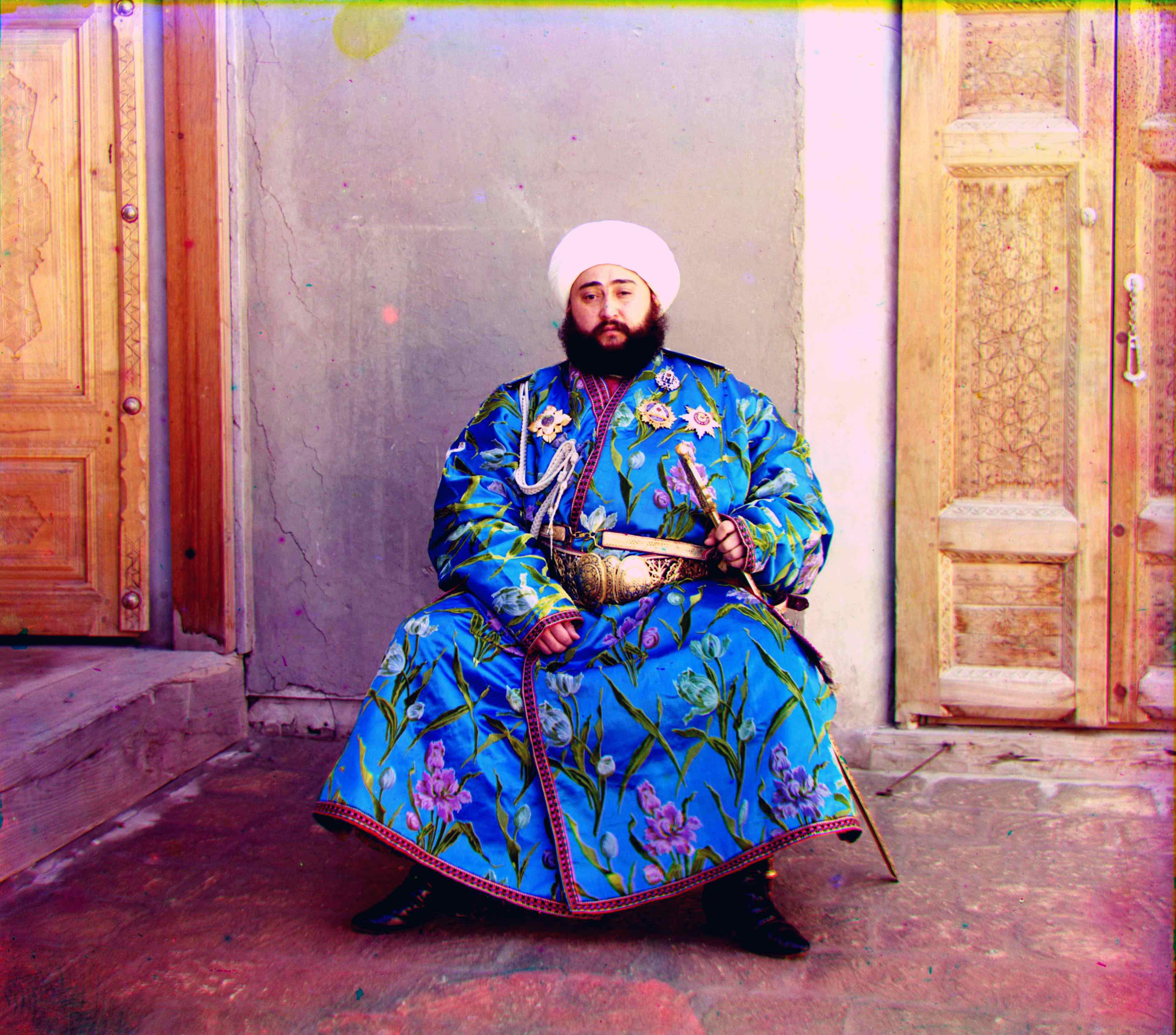
Output of Canny Edge Detection (emir)
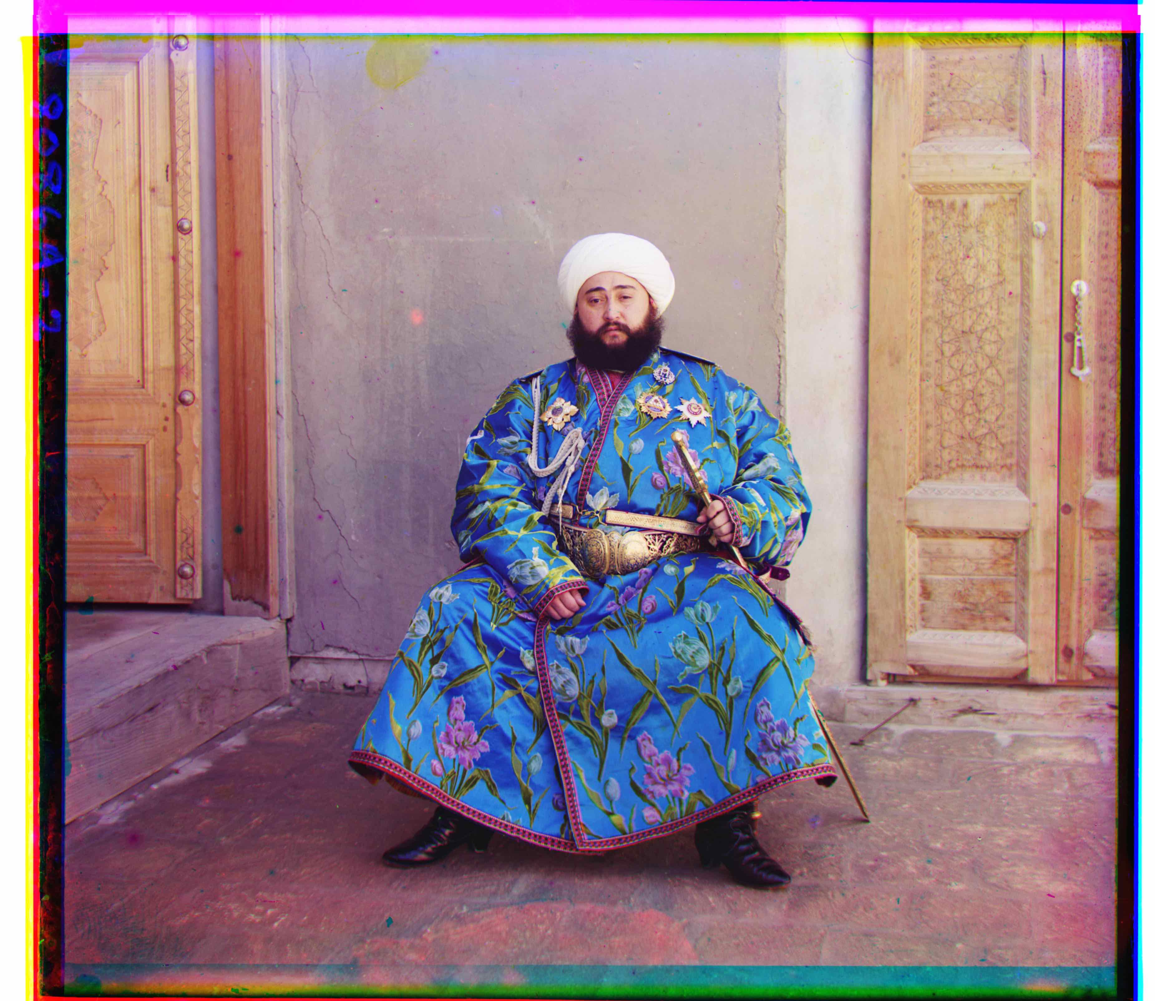
emir: final result using edge detection to find the displacement
great improvement from the previous one

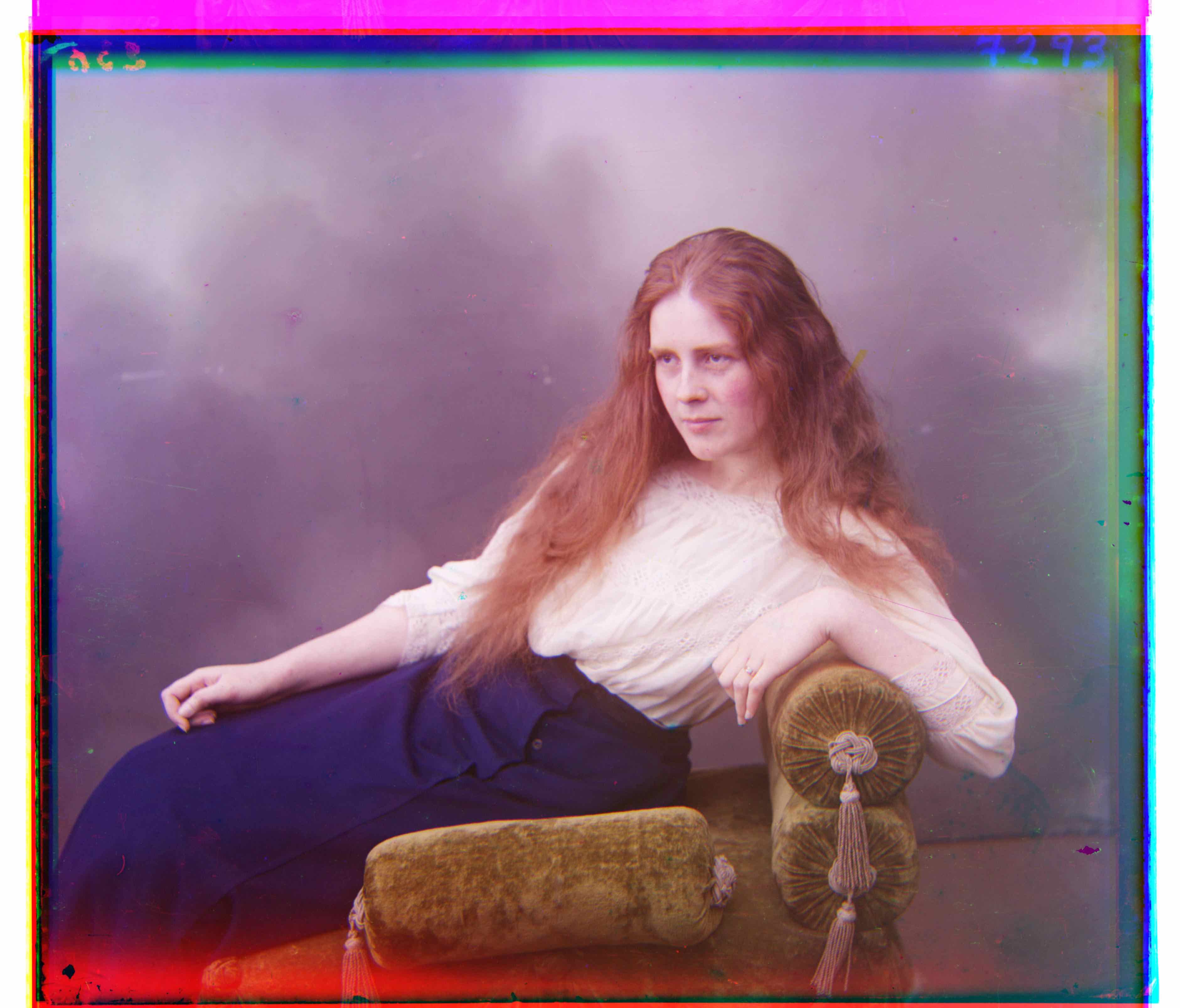
lady: using previous algorithm
lady: using edge detection
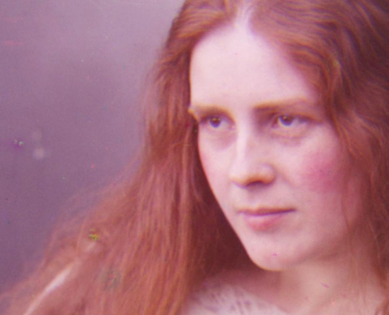
lady: using previous algorithm
lady: using edge detection
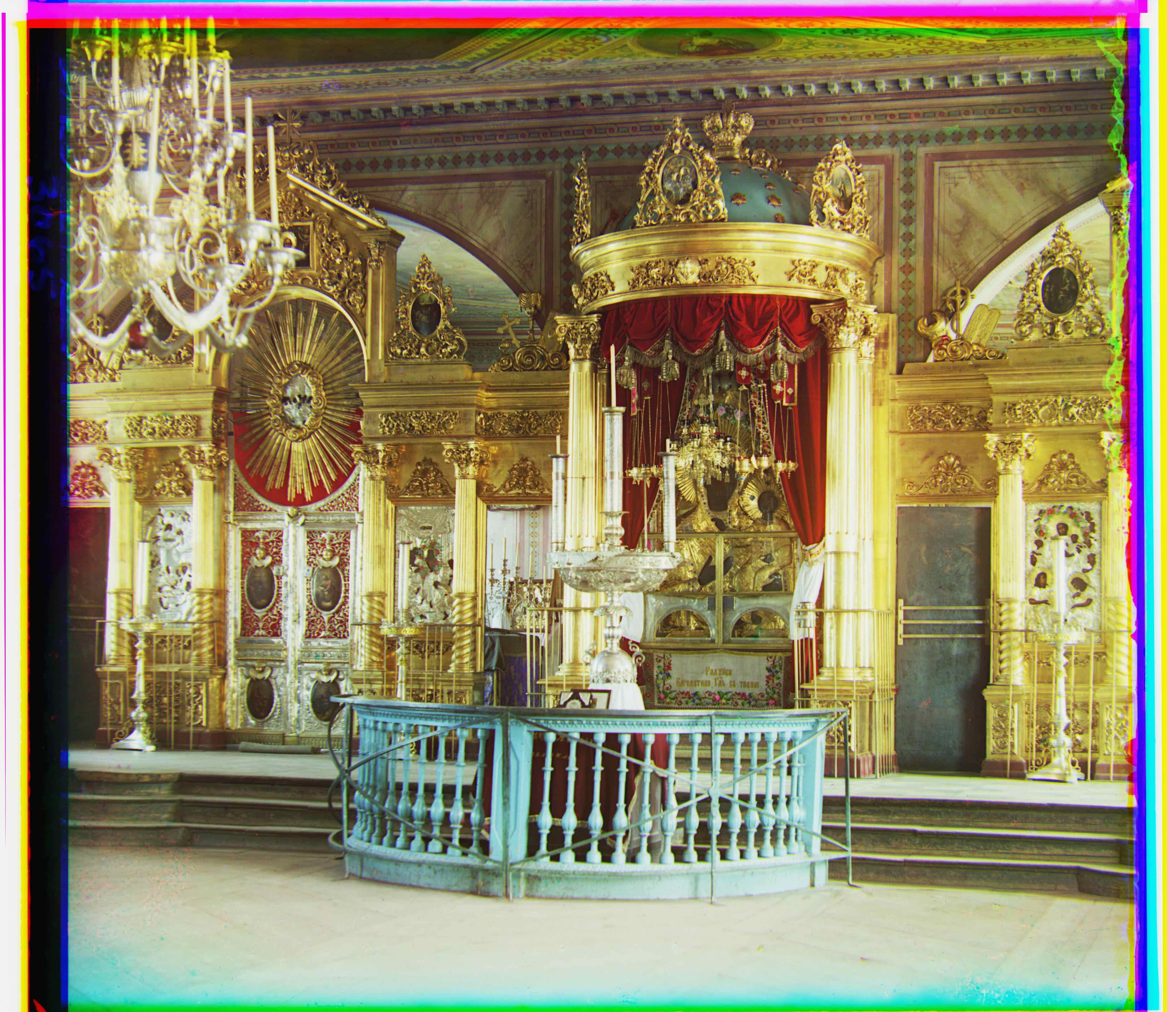
We can see that the icon one does not change much, but the lady image's quality decreases. Possibly because that the color of the lady is too similar to the environment thus it's not easy to detect the edge accurately.
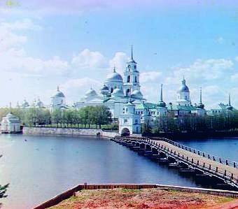
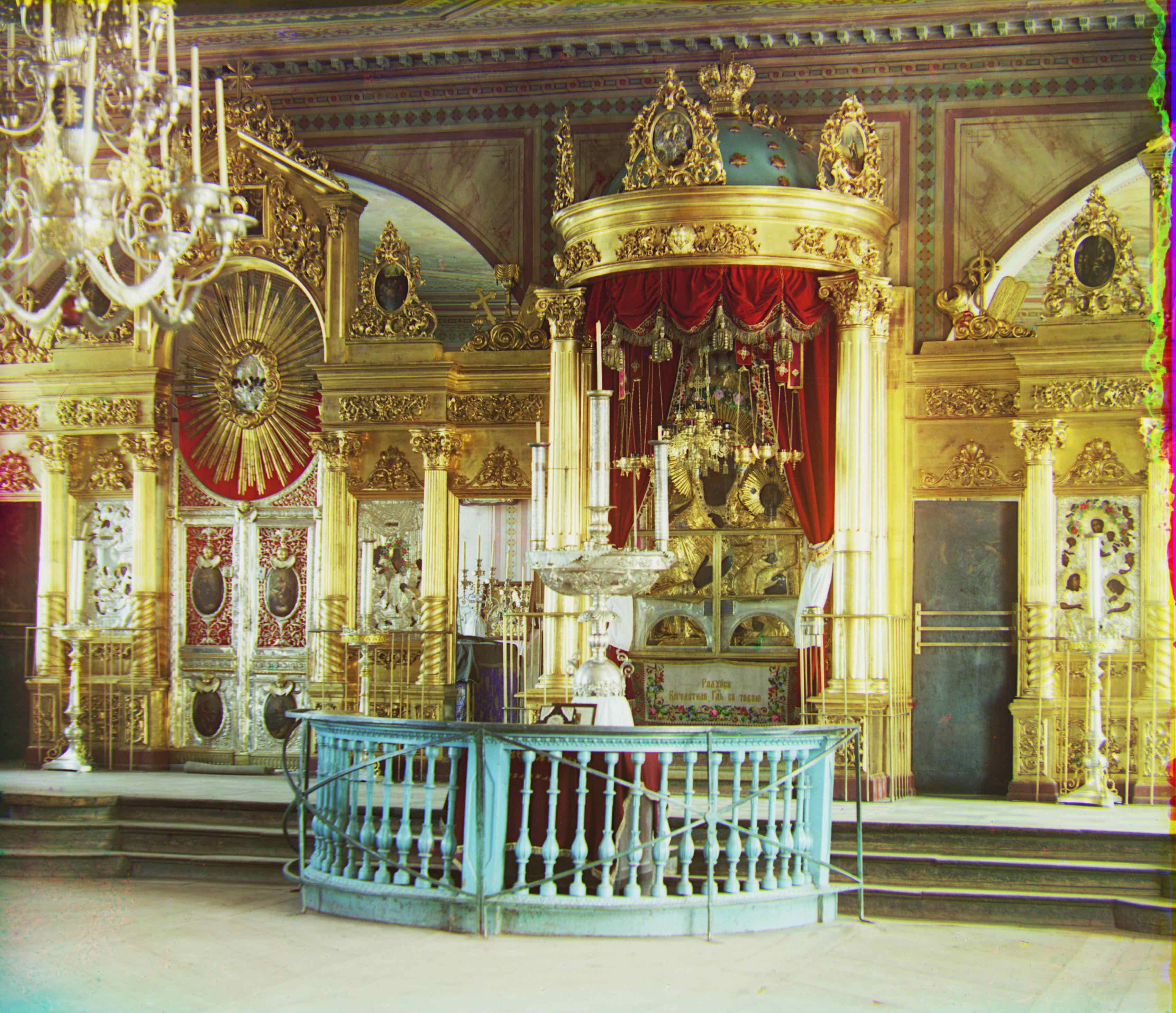
icon: using previous algorithm
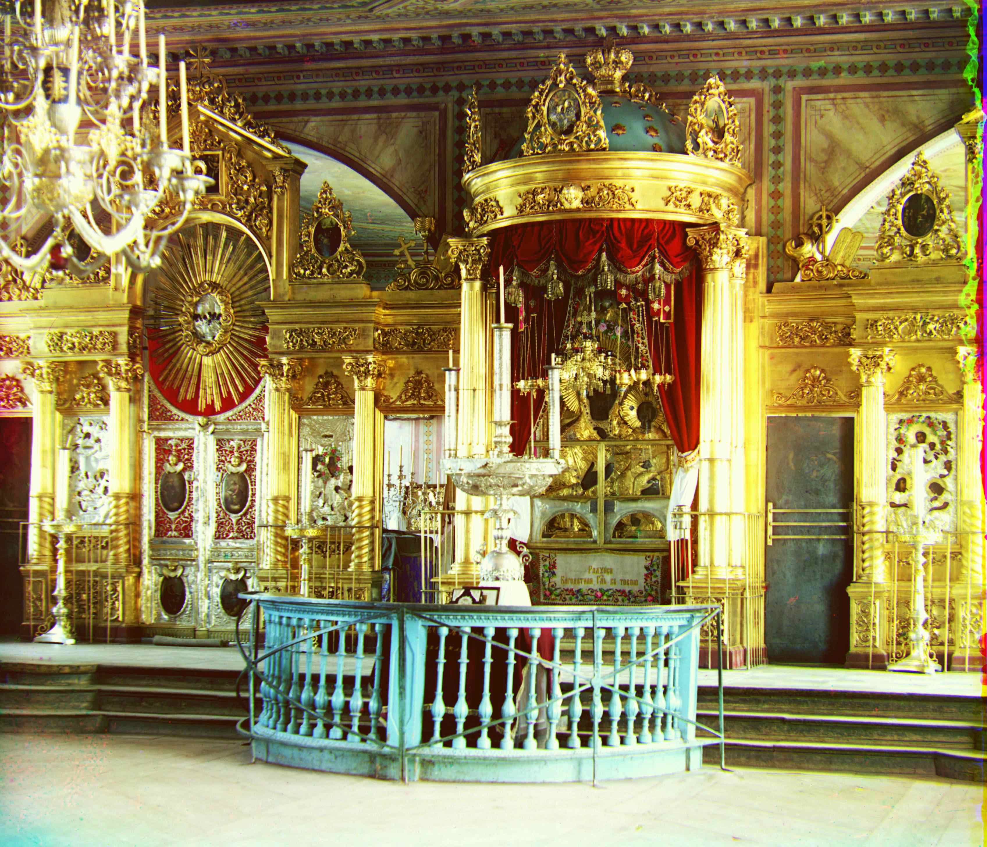
icon: using edge detection
Automatic cropping
The colored border in the outputs, whether in black, bright green, pink, or yellow, are quite annoying so an automatic cropping step is necessary. The algorithm I figured out is very simple and needs further improvement. Since the border usually have very low variance in color, at least a lot lower than its inner neighbors. I first separate a colored image’s R, G, B, values to three arrays and calculate the variance in each column and rows for each color separately. Then roll the arrays by 1 pixel. Use the original array to subtract this one then get the variance difference. The border must have a great difference value, but it’s not necessarily the maximum. Thus, I search over a predefined region, compare the top largest values and pick the inner one to crop. But those parameters should be determined more scientifically. Currently I just tried several times and choose reasonable ones. It works greatly for most of the images, but several stubborn borders still remains to be resolved.
Successful Examples
Before Auto Cropping
Before Auto Cropping
Before Auto Cropping
Before Auto Cropping
After Auto Cropping
After Auto Cropping
After Auto Cropping
After Auto Cropping
failure Cases
Before Auto Cropping
Before Auto Cropping
After Auto Cropping
After Auto Cropping
The parameters directly influence the outputs. If the searching area is not large enough, we will not be able to crop the whole border, but if it is too large, it will be possible to crop the parts that does not need to be cropped. Also, if we compare the indices of too many columns/rows with large variance, maybe we will eventually choose a column/row that is not a border at all. Thus, trying to find the properest parameters is the most important for this algorithm.
White Balancing
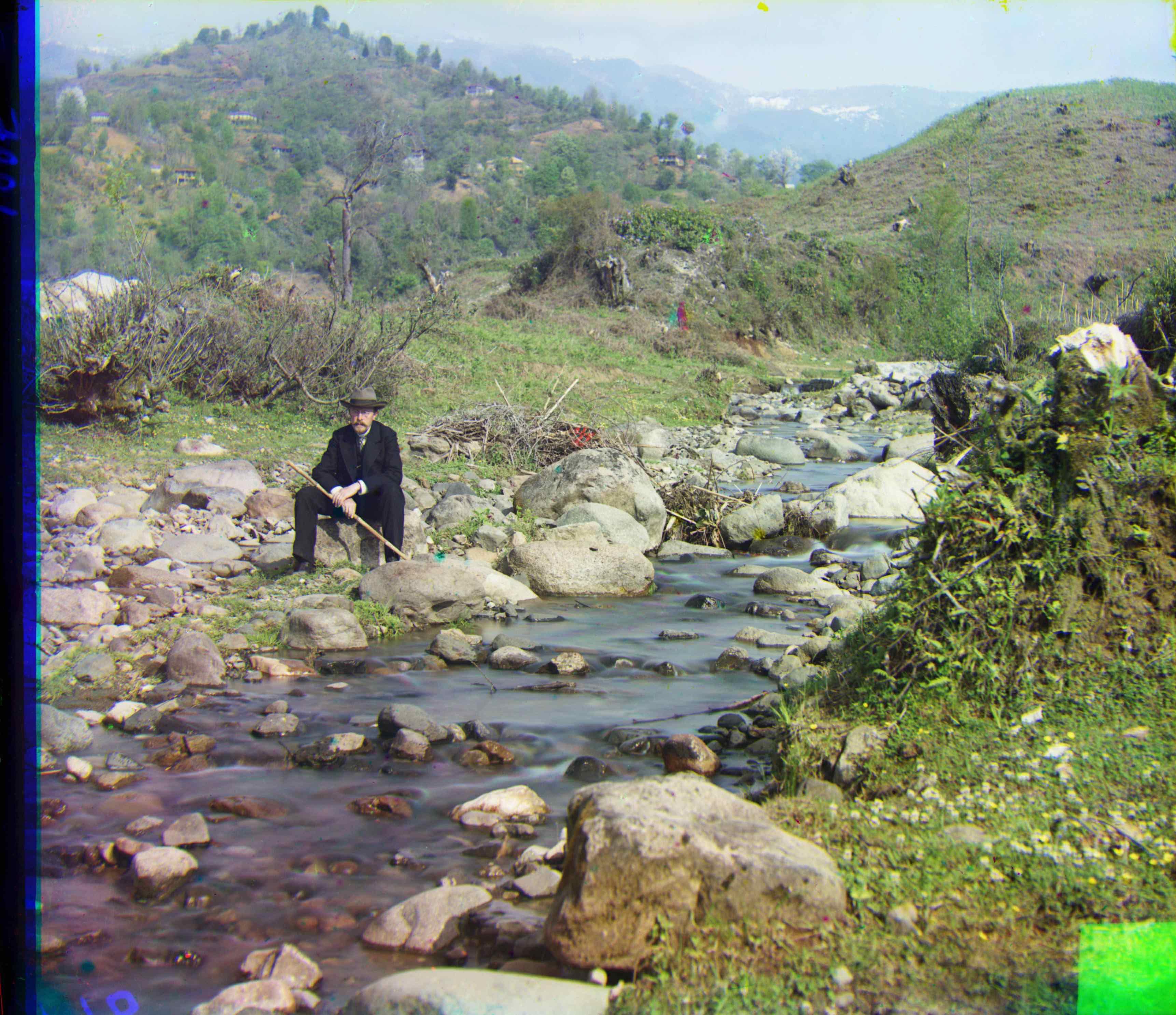
White balancing process makes a picture more realistic. Inspired by the method in this page: https://docs.gimp.org/en/gimp-layer-white-balance.html, my algorithm also discards the color values appears only 0.05% in the whole image and normalize the remaining graph. Here I use the normalizing method in cv, and the improvements are shown below:
Before White Balancing
Before White Balancing
Before White Balancing
Before White Balancing
After White Balancing
After White Balancing
After White Balancing
After White Balancing
Further Improvement
The white balancing process above use the normalization function in cv2. However, there are many kinds of ways to normalize our image arrays, for example calculating the Frobenius norm or Spectral norm as inspired by Taesung Park. In further experiments, I should try these different ways and figure out which one behaves the best in the white balancing process.
Final Results

Green: (5, 2)
Red: (12, 3)
Green: (48, 23)
Red: (106, 41)
Green: (-3, 2)
Red: (3, 2)
Green: (7, 0)
Red: (14, -1)
Green: (3, 1)
Red: (8, 0)
Green: (50, 15)
Red: (109, 14)
Green: (58, 3)
Red: (113, -3)
Green: (77, 29)
Red: (175, 37)
Green: (64, 13)
Red: (136, 23)
Green: (42, 6)
Red: (85, 32)
Green: (41, 18)
Red: (90, 23)
Green: (59, 18)
Red: (123, 15)
Other Examples

Green: (37, 21)
Red: (76, 36)
Green: (1, 0)
Red: (7, 0)
Green: (3, -1)
Red: (14, -3)
Green: (6, 3)
Red: (13, 4)
Green: (56, 22)
Red: (117, 29)
before edge detection:
Green: (52, 8)
Red: (112, 12)