Proj 3: Frequencies and Gradients

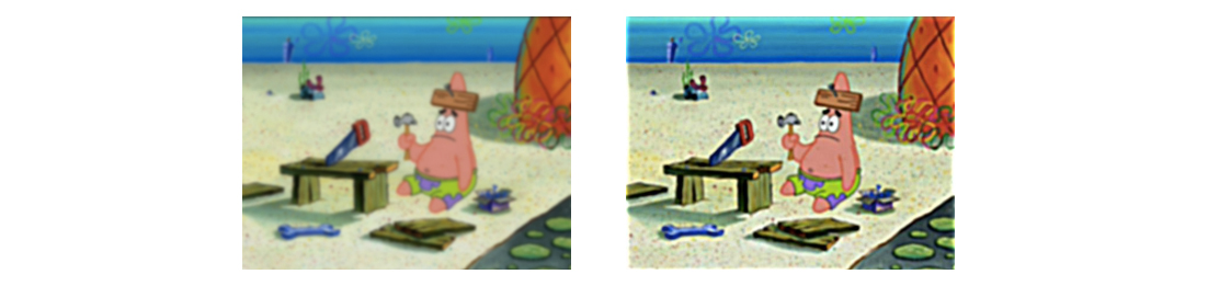
1.1 Warmup

First off, I tried to make Patrick from Spongebob sharper, because sometimes he's not that sharp.

1.2 Hybrid Images

To hybridize images, we add a lowpass version of one image to the highpass version of another. The detail can be seen as the difference between the original image and its lowpass version.

1.2 Image 1: Girl + Alien

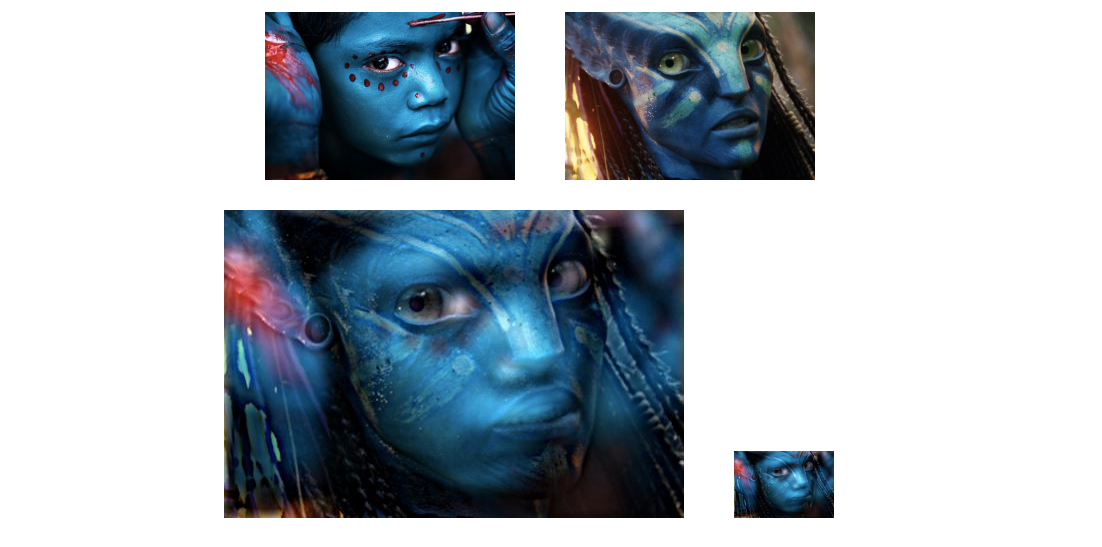From far away, you can see the portrait of a girl I got from Nat Geo. From up close, you see the protagonist of Avatar.

1.2 Image 2: Model + Dog

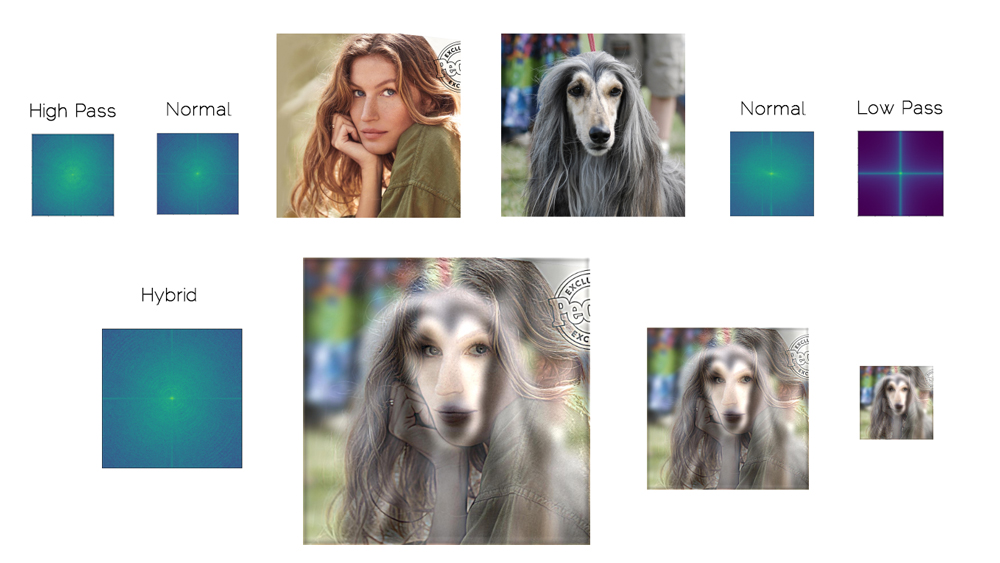
Doesn't Giselle Bundchen look great?

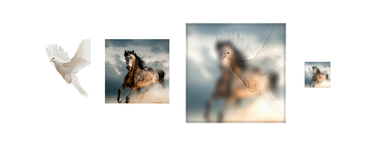
1.2 Image 3: Horse + Dove = Pegasus ?

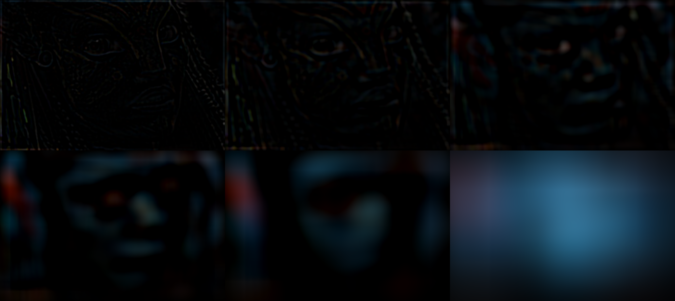
1.3 Laplacian and Gaussian Stacks

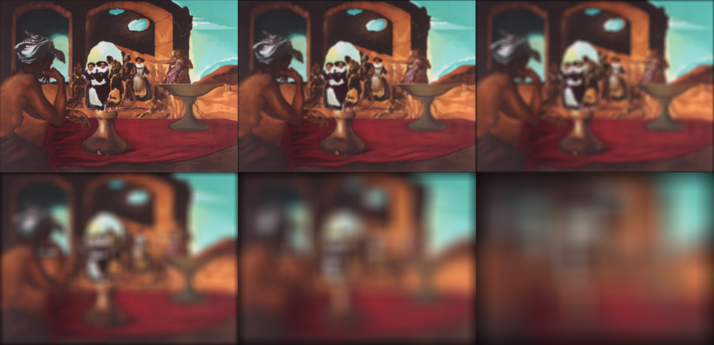
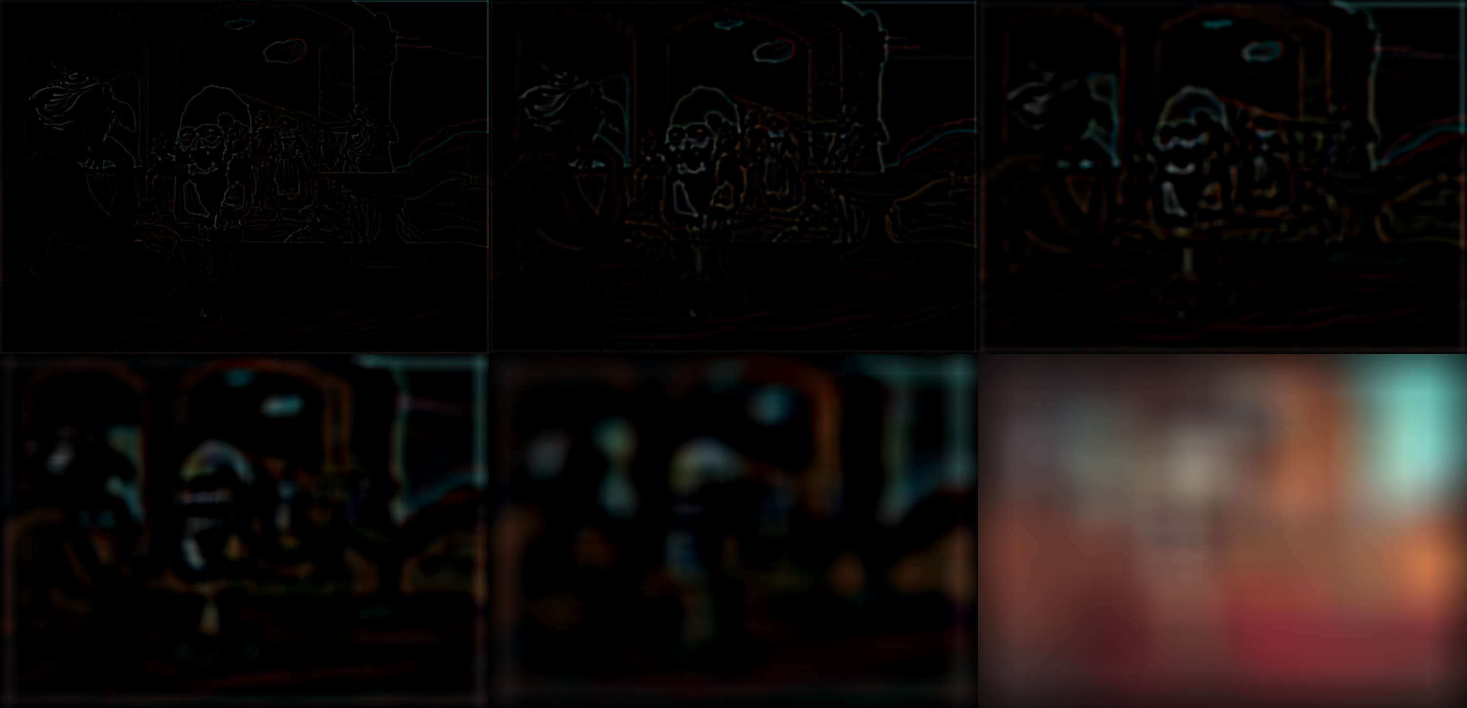
The image I chose to deconstruct was Dali's Slave Market with the Disappearing Bust of Voltaire. As we get blurrier, we see more of the Voltaire in the gestalt of the painting. In the Laplacian, going from right to left, we see more of the detail that defines the slave market.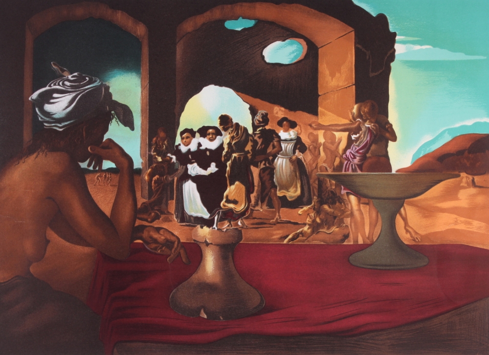 The hybrid image of mine that I chose to deconstruct was the Girl + Alien one. As you can see, going from left to right (higher to lower frequency), we see more of the girl in the first image (Gaussian stack). Going from right to left on the bottom image (Laplacian stack), we see more detail from the Avatar character.

1.4 Laplacian Blending

To implement Laplacian blending, I created gaussian stacks of the source image, the target image, and the mask. From the gaussian stacks of the source and target, I created laplacian stasks. Then for every layer in the stack, I computed a blended image as per this formula.

What this formula says is that at level j in the stack the j^th Laplacian of the source image will be weighted by j^th Gaussian of the mask (i ), and the j^th Laplacian of the target image at that level will be weighted by (1-the j^th Gaussian of the mask).

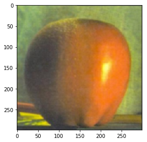
1.4 Image 1: My orapple.

1.4 Image 2: Me and what I should be for halloween: a satyr.

1.4 Image 3: Blending my mom and aunt together.

I blended my aunt's face with my mom's face, but then I realized there was no point because they are twins in the first place. If you look hard you can see that my mom (right) is not squinting, because the right side of her face has been replaced with my aunt's. But I bet you can't tell. Haha.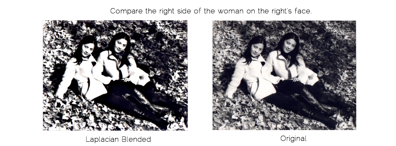

1.4 Image 4: Colorizing my mom with my mom.

I also messed with more of my mom's old photos. Here is a blended image that involves colorizing, blending, and two faces coming together. Wow. It's like 3 projects in 1.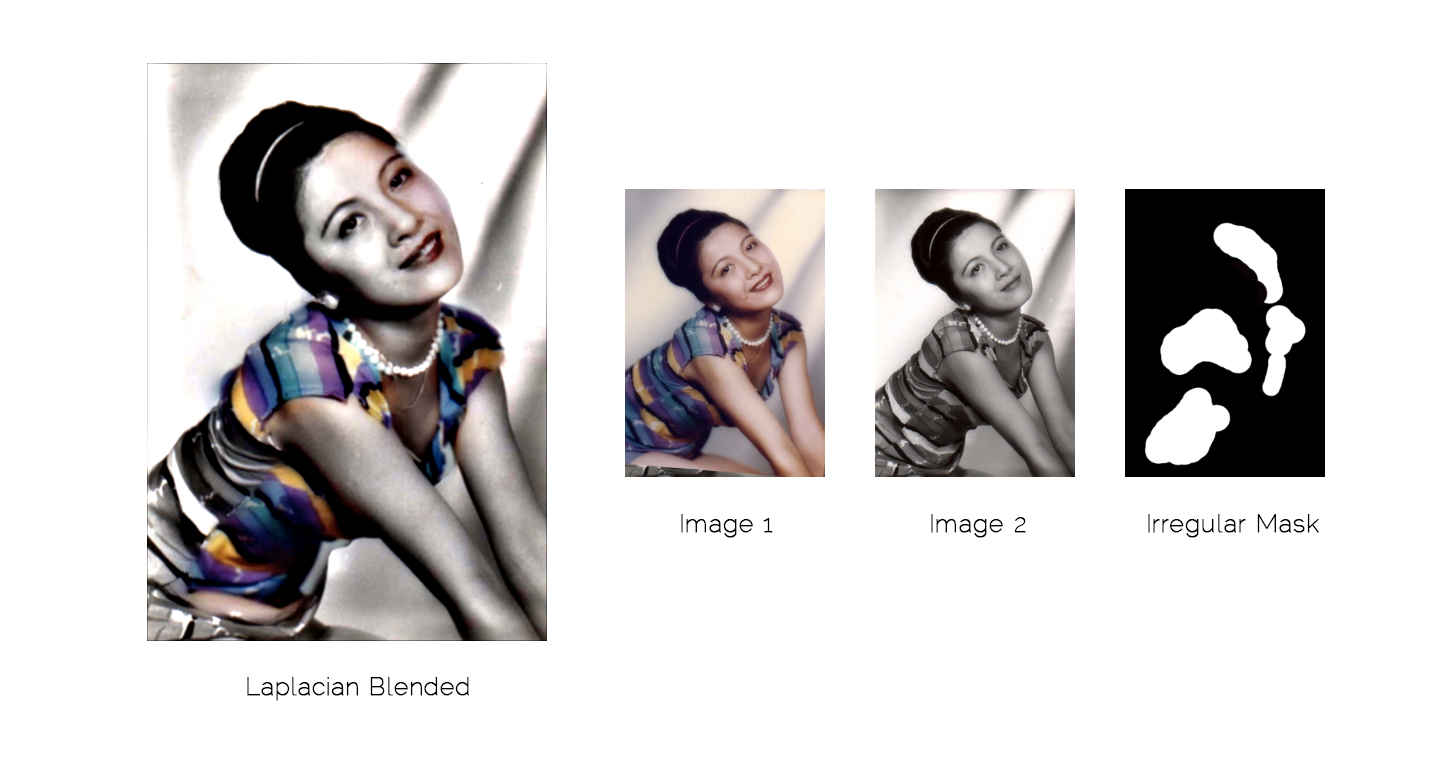

1.4 Image 5: Me plus Pillsbury Dough Boy.

At 2AM, I thought it would be a great idea to make Pillsbury Dough Boy dance in the sky in the background of a panorama where I look pretty pensive. You know, to lighten the mood. I ripped the source images from the frames of a youtube video and created a bunch of masks on Photoshop.

2.1 Toy Problem

2.1 Gradient Blending

Gradient blending requires a source, a target, and a mask. The algorithm uses least squares (Ax = b) to solve for the pixel intensity of the white areas in the mask (x).

First I created a sparse matrix that was ((mxn, mxn)) to represent A, the coefficient matrix of the system of equations. This matrix was only nonzero on the diagonal and in the four neighborhoods around the masked indices. The diagonals were nonzero because each pixel has an intensity to be solved for, even if the pixel is outside the mask and the value comes directly from the target image.

The 'four neighborhoods' were represented as coefficients/rows in the sparse matrix, with a 4 at the masked pixel and -1's for every neighbor also in the mask.

Then I constructed the 'b' vector either by computing the four neighborhood from the correct image or copying the value over from the target image (if the pixel was outside the mask). By the four neighborhood from the correct image, I mean the src image if the entire four neighborhood around the masked pixel is also in the mask and the target image otherwise.

The challenging part about this implementation was that it could get computationally expensive really fast depending on the size of the mask, so the code had to be vectorized.

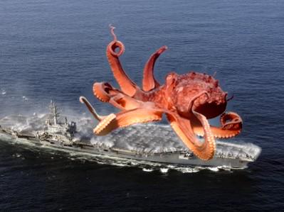
2.2 Image 1: My attack octopus.

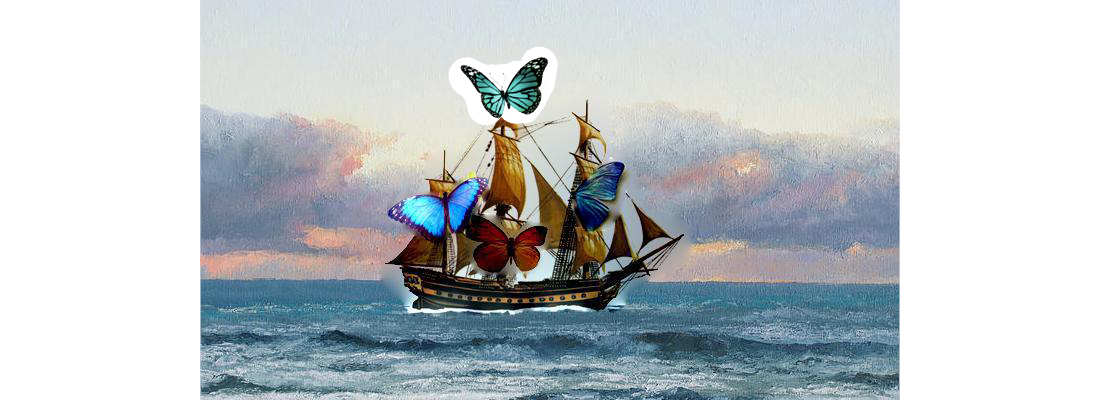
2.2 Image 2: Hive Gave Me Butterflies

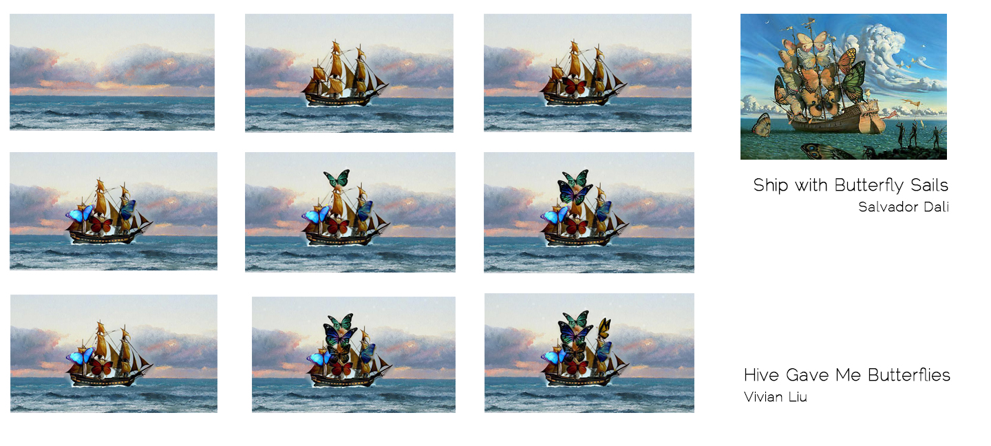
I titled it Hive Gave Me Butterflies, because Hive9, Hive11, and Hive30 really worked hard for me this weekend. Also, you get pretty antsy when your program runs for a long time.

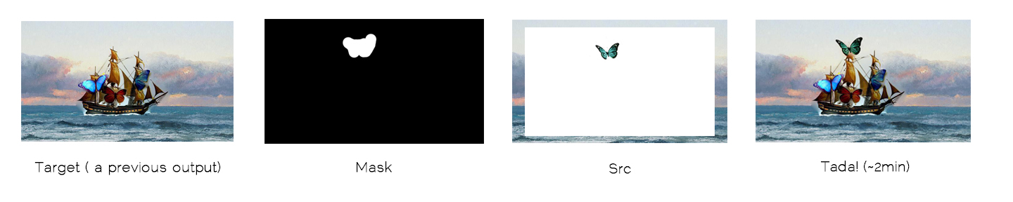
You can see above here the type of mask, source image, and target image I used to construct this, as well as how it looks just copy and pasted. Each color channel took approximately 20-40 seconds.

2.2 Image 2: My Dog Time Traveling to my Mom

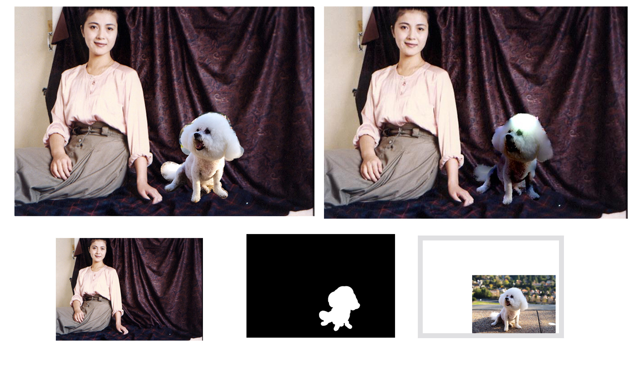
A failure case: I believe the reason why this one failed is because the gradients (the curtains, the backyard my dog came from) were too dissimilar to match properly.

2.2 "So you wanna be on top?" - America's Next Top Model's slogan.

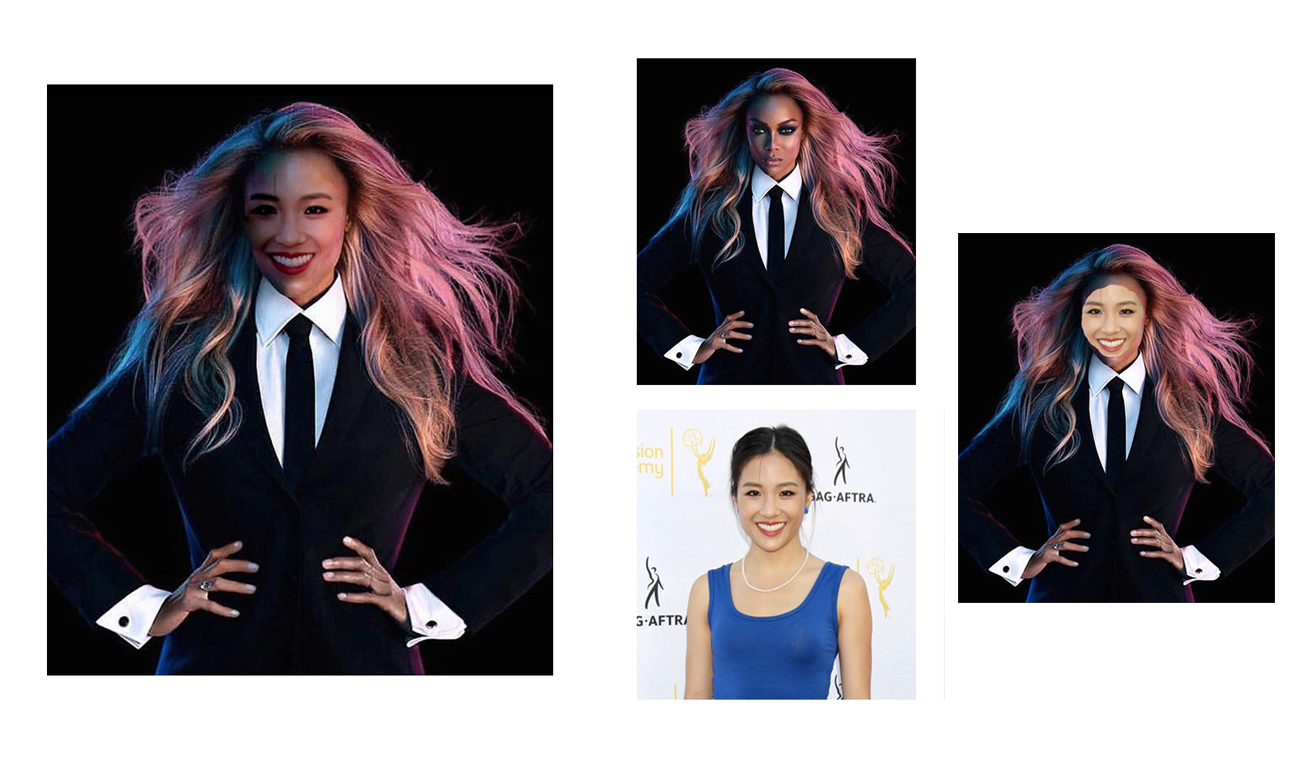
Another failure case: I think this one failed because of the same deal, the lighting on the left side of the face is more dramatic and contrasted too much with the even, well-lit nature of the source image.

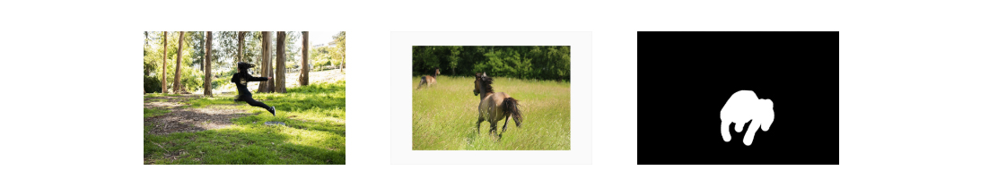
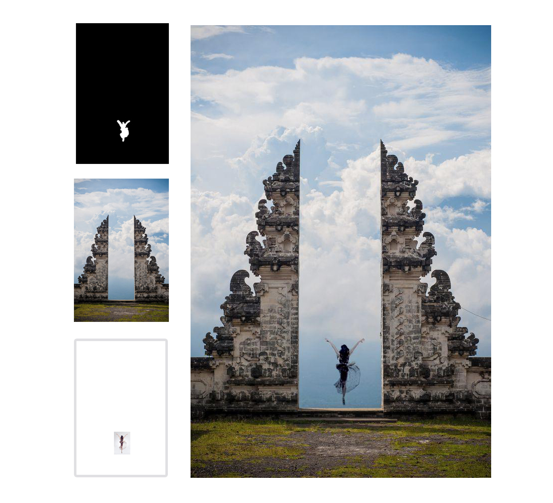
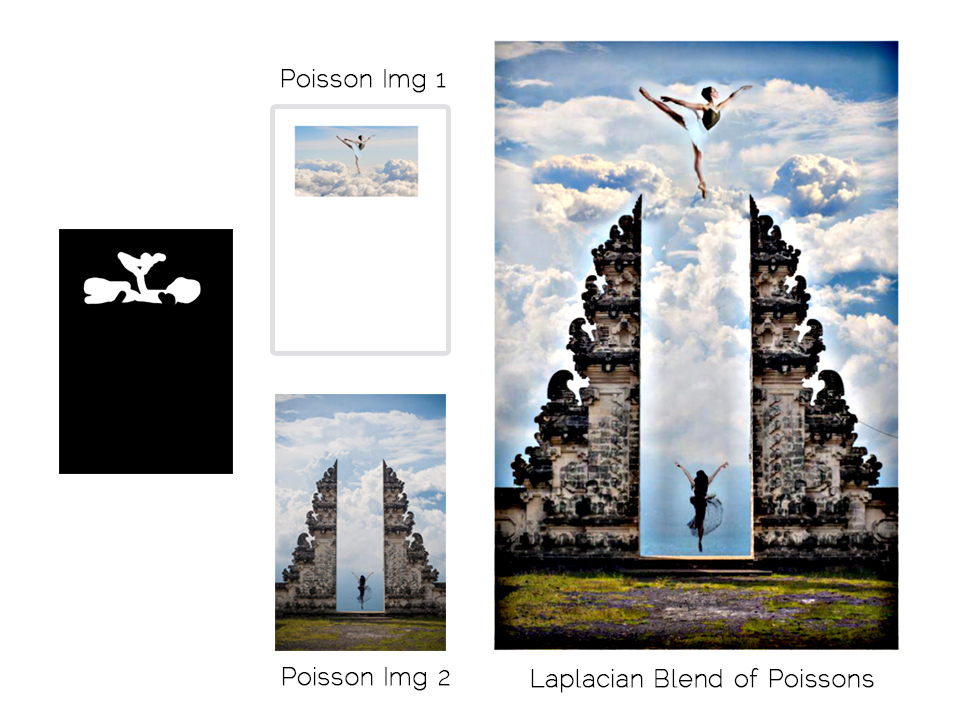
2.2 Image 4: Dancing in Indonesia

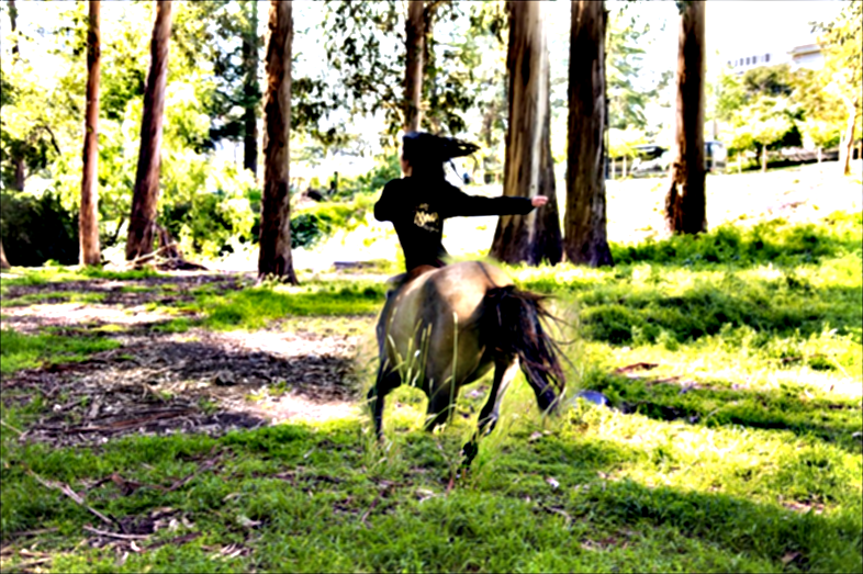
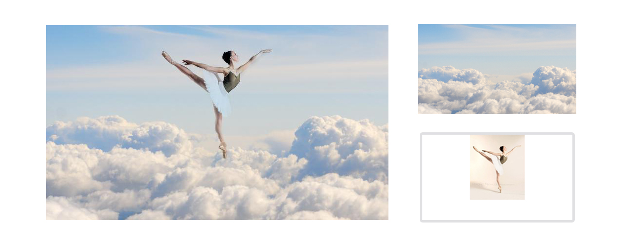
2.2 Image 5: Aerial Ballet

2.2 Image 6: Hybrid on hybrid.

I wasn't really impressed with the previous two images (the ballerina and the contemporary dancer), so I thought I might as well Laplacian blend the Poisson outputs together to see if I could create a better manipulation. The nice thing to note is that the clouds copied over so nicely from the ballerina image that I had to look quite carefully to notice the difference!

Poisson vs. Laplacian Reflection

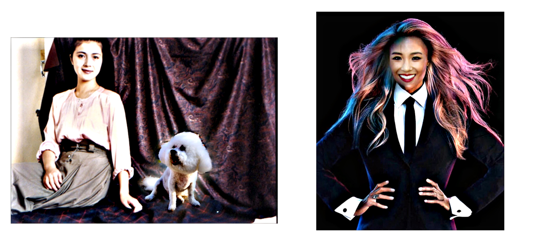
Putting speed aside (Poisson blending took far longer), the Laplacian blending preserved the color of the source image better even when the source and the target had too much contrast by the boundaries. As we can see in these two images (which were fails for Poisson), the luminance of my dog and Constance Wu (the src images) are unaffected by the dark backdrop of the curtains (left) and the dramatic lighting (right).

However, the tradeoff is that the target and the source no longer blend as seamlessly. For my dog, you can still see specters of the background he came from.

Basically, Poisson blending is worse when the gradients and the boundaries are drastically different from each other. Laplacian blending is worse when you really want the seamless transition between source and target that Poisson guarantees.

If you can't tell, I had fun. Thanks for reading!