CS 194-26 Project 3: Frequencies & Gradients
Jennifer Liu (cs194-26-aag)
Part 1.1: Warmup
The image I showed to sharpen is of 2 dogs. Here is the original:
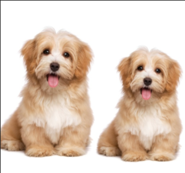
After sharpening, it looks like this:
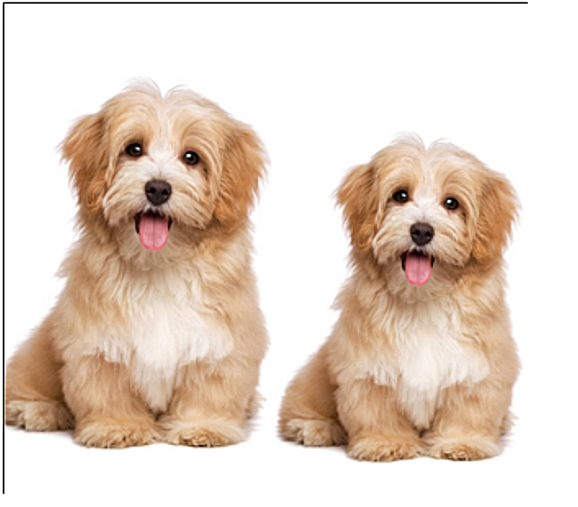
To create the sharpened effect, I applied a Gaussian kernel on the original dogs image. Then, I subtracted the smoothed image from the original image to get the detail. To obtain the sharpened image, I then added the detail to the original image.
Part 1.2: Hybrid Images
In this part, I created hybrid images by low-pass filtering one image with the Gaussian, and high-pass filtering another image with the Laplacian, and then combining the two images together.
Here are a few results:
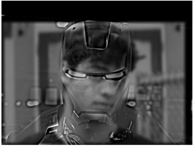
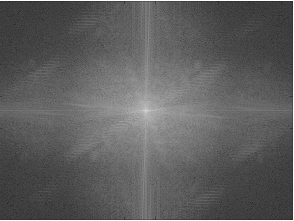
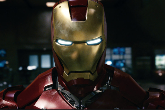
This is Peter Kavinsky hybridized with Iron Man, two of my favorite people. The frequency analysis shown is for this image.
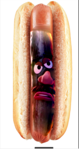
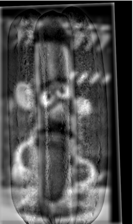
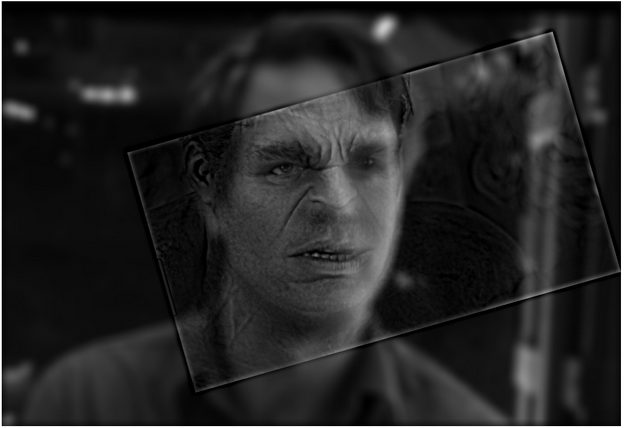
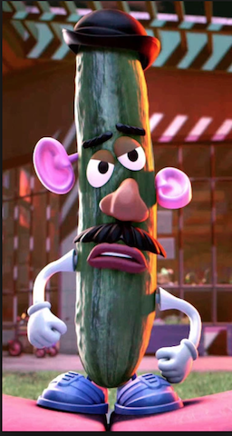
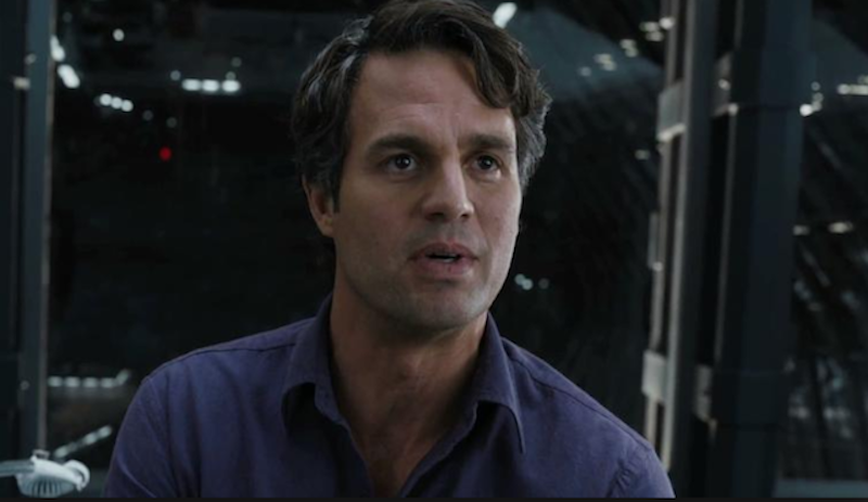
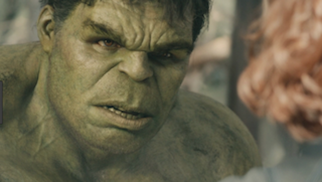
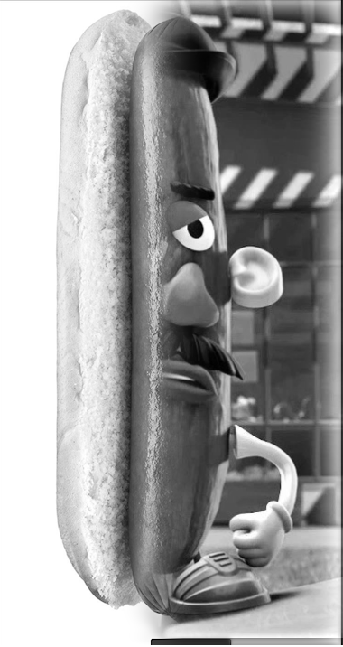
These next two images are of Mr. Potato Head when he was a cucumber and a hot dog hybridized, and Mark Ruffalo and the Hulk hybridized together.
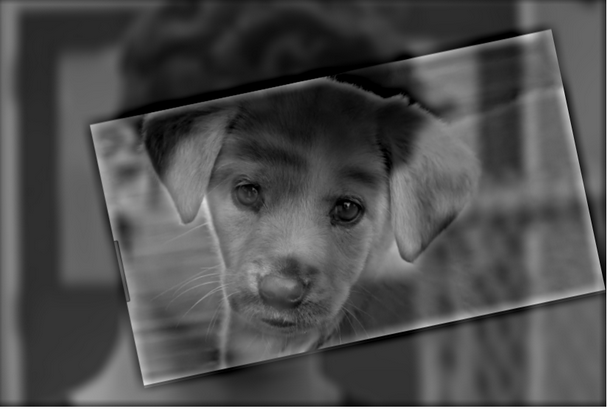
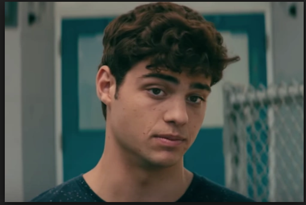
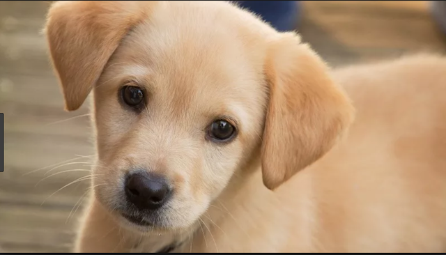
This next one I consider a failure, since the shapes of the faces of Peter Kavinsky/Noah Centineo do not align well with that of a puppy:
For reference, here are the original images:
Part 1.3: Gaussian & Laplacian Stacks
In this part, I implemented Gaussian and Laplacian stacks by recursively applying either a Gaussian kernel or recursively performing the procedure for the Laplacian (Image - Guassian(Image)). Here are the results when applying a Gaussian stack and Laplacian stack with 5 levels each on the Dali painting:
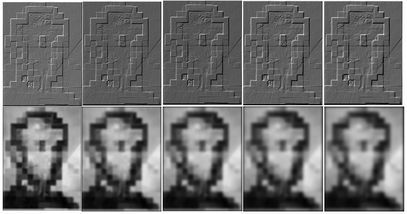
You can see that repeatedly applying the Gaussian makes the image more blurry as we increasingly smooth the image, and makes Abraham Lincoln more prominent and the girl in the image less noticeable. In the Laplacian stacks, however, the girl's outline becomes much more visible and you can no longer see Abraham Lincoln.
Part 1.4: Multiresolution Blending
In multiresolution blending, I created a blended image by creating gaussian and laplacian stacks for two images I'll call image1 and image2. In addition, I created a mask that consisted of half zeroes and half ones divided vertically, and created a gaussian stack for the mask. Then, at each level, I created a blended laplacian stack from the equation Lblend = Gmask*(L1)+(1-Gmask)*(L2). Adding the blended laplacians together yields the smoothly blended images you can see below. The smoothness is a result of incorporating the smoothed mask at each level into the summation between the laplacians for image1 and image2 at that particular level.
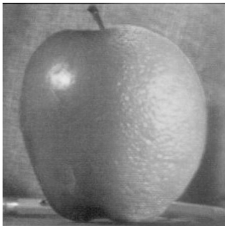
Here is the apple and orange blended together as seen in lecture:
Here's an image of the previous hot dog blended with the previous Mr. Potato Head on a cucumber from Toy Story 3:
Part 2 Overview: In this part, I investigated blending images together by trying to minimize the gradient (the amount of change) in between the boundaries of a source image and target image, as well as within the source image that we want to insert into some specified background image. To do this, we want to solve for the pixel values within the masked region (where the source image will be inserted into the background) by formulating a least squares problem that preserves (as closely as possible) the difference in pixel values in the source image, and match the difference in pixel values between a boundary pixel in the mask region of the source image and its neighboring pixel in the background image with the pixel difference between the pixels in the corresponding positions within the source image.
Part 2.1: Toy Problem
This toy problem was meant to help us familiarize with implementing the gradient domain processing. I solved for v to reconstruct the toy image by minimizing the difference between the x gradients within v and the x gradients within the toy image as well as the y gradients within v and y gradients within the toy image. In addition, an extra constraint was enforced: the top left pixel in v had to match the top left pixel in the toy image. Since the minimum error would be if the pixel values in v were exactly the same as that of the toy image with this additional constraint, v is simply a reconstruction of the toy image with a very, very small error on the order of 10^-6.
Here is the original image:
Here is the reconstructed image:
Part 2.2: Poisson Blending
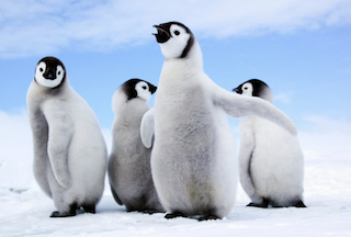
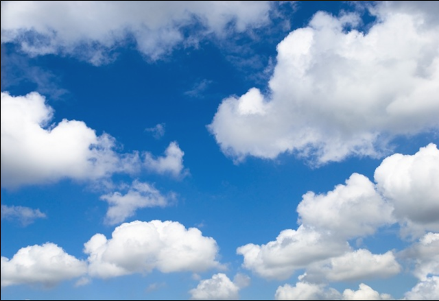
In the final part of the project, I implemented poisson blending to (ideally) seamlessly blend a small part of a source image (a penguin in the below example) into a background image (the sky). This was done by using least squares to solve for the best pixel values to fill in to the masked region within the background image, such that the gradient within the blended image would be as close as possible to that of the source image within the masked region. In addition, the gradient between the boundaries of the masked region and the background image was also minimized to be as close to the gradient within the corresponding pixels in the source image. Figuring out how to utilize sparse matrices to improve the speed of the algorithm was the most difficult part of the project, as the least squares solver would run for quite a while without it.
This blending result of a penguin on a cloud was my favorite.
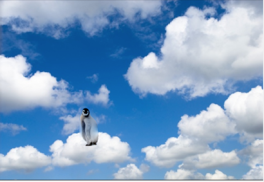
Here's the source and target images for it:
Here are some additional results, of varying success:
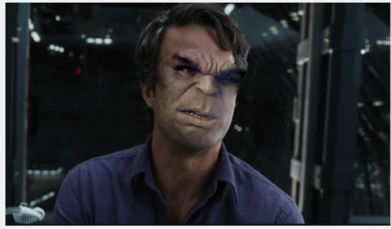
I think this one didn't work so well because Hulk's face was slightly too big, and I couldn't get it to be exactly the right angle... also, there's a slight difference in the textures of their skin, which also made blending slightly less than optimal.
I also blended the hot dog and Mr. Cucumber from before once again, but it didn't work out so well because of the huge difference when the image is in color. I think if the image was in grayscale, it would have turned out better in this case. I think poisson blending is good for when the colors of the images to be blended are relatively similar in hue and shade, and if the textures are similar.